Content from Python Basics
Last updated on 2024-11-27 | Edit this page
Estimated time: 30 minutes
Overview
Questions
- Why should I use Python?
- How should I use Python?
- What basic object types can I work with in Python?
- How can I create a new variable in Python?
- How do I use a function?
- Can I change the value associated with a variable after I create it?
Objectives
- Understand the general motivation for Python and appropriate use cases.
- Assign values to variables.
If you are using a Jupyter notebook to run the examples, the keyboard shortcut, shift+enter, will evaluate a cell and generate output.
Python
Python was first released in the early 90s by Guido von Rossum, a Dutch programmer who was looking for a hobby project when his government-run research lab in Amsterdam had closed for the holidays. As further noted in his foreword for “Programming Python,” Guido named the programming language after Monty Python’s Flying Circus and wanted a high-level scripting language that would appeal to Unix and C programmers.
He had spent a lot of time thinking about the problems of existing high-level programming languages and decided Python should address many of his concerns. The result is something that aims to create readable, reusable, fast-to-write flexible code that values the programmer’s time in generic tasks over the raw performance of the interpreter’s execution. That is, for a specific compute task, pure Python will typically be slower than an alternative, specialized framework. However, a programmer that knows Python will be equipped to quickly write an understandable solution. In the cases where Python’s computation is too slow, the ability to quickly build a prototype is still invaluable.
Python is dynamically typed, garbage-collected, and supports
object-oriented, procedural, and functional programming paradigms. In
Python, most variables are instances of objects and often times people
will say, “in Python, everything is an object.” The dynamic typing is
also commonly called “duck
typing,” as the interpreter determines whether to encode symbols
like the number 5 as an integer object and the number
5. as a floating-point object based on the presence of the
decimal point or the larger context of the arithmetic, “…if it quacks
like a duck…”
In a scientific computing setting, one last point that makes Python competitive to other high-level languages, like MATLAB or Julia, is that it is very easy in Python to wrap existing frameworks. Thus, Python becomes an exceptionally convenient medium for moving data between already existing and performant scientific libraries, with the programmer “minimizing” the use of Python built-ins to solve problems. This ability to act as a “scientific library glue” has made Python one of the most popular programming languages within the scientific community and allows Python to be just as compute-performant as the more specialized frameworks of MATLAB and Julia.
By the end of this tutorial, attendees should have a familiarity with
basic Python, common performance libraries like numpy,
common plotting libraries like matplotlib, and via a simple
example, how to wrap external libraries.
Variables
Any Python interpreter can be used as a calculator:
OUTPUT
23This is great but not very interesting. To do anything useful with
data, we need to assign its value to a
variable. In Python, we can assign a value to a variable, using the equals sign
=. For example, we can track the weight of a patient who
weighs 60 kilograms by assigning the value 60 to a variable
patient_weight_kg:
From now on, whenever we use patient_weight_kg, Python
will substitute the value we assigned to it. In layperson’s terms,
a variable is a name for a value.
In Python, variable names:
- can include letters, digits, and underscores
- cannot start with a digit
- are case sensitive.
This means that, for example:
-
weight0andweight_0are a valid variable names, whereas0weightis not -
weightandWeightare different variables
Stylistic Note
Real world variables are typically given multi-word names to improve
code legibility. For instance, patient_weight_kg instead of
just w or kg communicates to code readers that
the variable stores a weight in kilograms for a patient. The use of
underscores in the variable name like patient_weight_kg is
an example of snake case, which is the cultural style of
Python.
Common object types
In Python, nearly every variable is an instance of some class, which provide powerful builtin methods for transforming the underlying object. We start simple, by introducing three common “variable types”:
- integer numbers, which are
intobjects, - floating point numbers, which are
floatobjects, - strings, which are immutable
strobjects.
In the example above, variable patient_weight_kg is an
int object with an integer value of 60. It is
not possible to define an int object’s value with anything
other than an integer number. If we want to more precisely track the
weight of our patient in kilograms, we can use a floating point value by
executing:
Challenge
Why is the float patient_weight_kg = 60.3
less precise than the int
patient_weight_g = 60300?
Floating-point arithmetic results in rounding errors. The default floating-point computer number uses 64 bits to store values, such that 1 bit stores a sign, 11 bits store an exponent, and the remaining 52 bits store the significand. This double precision system results in exactly \(2^{52}-1\) (roughly 4.5 quintillion) numbers exclusively between every representable power of 2, for instance, between 1/2 and 1, 1 and 2, or \(2^{100}\) and \(2^{101}\). The resulting finite rational number system is non-associative, for instance, letting \(\varepsilon=2^{-52}\), \((2+\varepsilon)+\varepsilon \neq 2+(\varepsilon + \varepsilon)\).
![Figure illustrating rounding errors for different values between 1 and 1 plus machine epsilon. Values in $[1+\varepsilon/2,1+\varepsilon]$ will be rounded up to the nearest computer floating-point number, $1+\varepsilon$; else values will be rounded down to $1$. When computing sums, higher-precision ***registers*** are used which then follow rounding rules when truncating to the lower precision floating-point.](../fig/floating-point-rounding-figure.png)
In a quirk of Python, base int integers allow arbitrary
precision.
To create a string, we add single or double quotes around some text. To identify and track a patient throughout our study, we can assign each person a unique identifier by storing it in a string:
Using Variables in Python
Once we have data stored with variable names, we can make use of it in calculations. We may want to store our patient’s weight in pounds as well as kilograms:
We might decide to add a prefix to our patient identifier:
Built-in Python functions
To carry out common tasks with data and variables in Python, the
language provides us with several built-in functions.
To display information to the screen, we use the print
function:
OUTPUT
132.66
inflam_001
When we want to make use of a function, referred to as calling the
function, we follow its name by parentheses. The parentheses are
important: if you leave them off, the function doesn’t actually run!
Sometimes you will include values or variables inside the parentheses
for the function to use. In the case of print, we use the
parentheses to tell the function what value we want to display. We will
learn more about how functions work and how to create our own in later
episodes.
We can display multiple things at once using only one
print call:
OUTPUT
inflam_001 weight in kilograms: 60.3We can also call a function inside of another function call. For example,
Python has a built-in function called type that tells you a
value’s data type:
OUTPUT
<class 'float'>
<class 'str'>
Moreover, we can do arithmetic with variables right inside the
print function:
OUTPUT
patient weight in pounds: 132.66The above command, however, did not change the value of
patient_weight_kg:
OUTPUT
60.3To change the value of the patient_weight_kg variable,
we have to assign
patient_weight_kg a new value using the equals
= sign:
OUTPUT
patient weight in kilograms is now: 65.0Variables as Sticky Notes
A variable in Python is analogous to a sticky note with a name written on it: assigning a value to a variable is like putting that sticky note on a particular value.

Using this analogy, we can investigate how assigning a value to one variable does not change values of other, seemingly related, variables. For example, let’s store the subject’s weight in pounds in its own variable:
PYTHON
# There are 2.2 pounds per kilogram
LB_PER_KG = 2.2
patient_weight_lb = LB_PER_KG * patient weight_kg
print('patient weight in kilograms:', patient_weight_kg, 'and in pounds:', patient_weight_lb)
OUTPUT
patient weight in kilograms: 65.0 and in pounds: 143.0Everything in a line of code following the ‘#’ symbol is a comment that is ignored by Python. Comments allow programmers to leave explanatory notes for other programmers or their future selves.

Similar to above, the expression
LB_PER_KG * patient_weight_kg is evaluated to
143.0, and then this value is assigned to the variable
patient_weight_lb (i.e., the sticky note
patient_weight_lb is placed on 143.0). At this
point, each variable is “stuck” to completely distinct and unrelated
values.
Let’s now change patient_weight_kg and introduce an
f-string (string with first quote prefixed with an f), a
fast way for Python and the programmer to interpolate strings with
potentially formatted variable values:
PYTHON
patient_weight_kg = 100.0
print(f'patient weight in kilograms is now: {patient_weight_kg} and weight in pounds is still {patient_weight_lb}')
OUTPUT
patient weight in kilograms is now: 100.0 and weight in pounds is still: 143.0
Since patient_weight_lb doesn’t “remember” where its
value comes from, it is not updated when we change
patient_weight_kg.
OUTPUT
`mass` holds a value of 47.5, `age` does not exist
`mass` still holds a value of 47.5, `age` holds a value of 122
`mass` now has a value of 95.0, `age`'s value is still 122
`mass` still has a value of 95.0, `age` now holds 102Sorting Out References
Python allows you to assign multiple values to multiple variables in one line by separating the variables and values with commas. This kind of syntax is called, multiple assignment. What does the following program print out?
OUTPUT
Hopper Grace
Noether EmmyBasic arithmetic operations
In Python, exponentiation of int and float
objects is done with the ** operator.
OUTPUT
2.7169239322355936Something quirky is that / is a true
divide whereas // does a floor
division, which will preserve ints but cast
to float when mixing types.
OUTPUT
1.3333333333333333 1 1.0 1.0The % computes a modulus
OUTPUT
0.7182816941320818 5Since most variables are objects in python, all operators may be
redefined, but this is generally not recommended. Instead, operators can
be leveraged to provide greater high-level functionality. For instance,
the builtin str class uses “multiplication” to quickly
generate a repeated string pattern,
OUTPUT
=~=~=~=~=~=~=~=~=~=~=~=~=~=~=~=~=~=~=~=~=~=~=~=~=~=~=~=~=~=~=~=~=~=~=~=~However, division is not defined.
OUTPUT
TypeError: unsupported operand type(s) for /: 'str' and 'int'A final operator to note is the matmul symbol,
@. This will be utilized in a later section when
introducing a powerful Python library called numpy.
Using external modules
Python is a Turing-complete programming language. This means that it is possible with Python to construct any arbitrary program. Often times, we want to build modules that serve as function libraries for us to leverage when tackling a problem. Additionally, as mentioned at the start of the lesson, Python is exceptional for its ability to wrap external, non-Python libraries and make them available within Python. To motivate this, consider the challenge of computing the natural logarithm of a number:
OUTPUT
---------------------------------------------------------------------------
NameError                                 Traceback (most recent call last)
Cell In[7], line 1
----> 1 log

NameError: name 'log' is not defined
As the error indicates, out-of-the-box Python does not know what we
mean by log — it is undefined. One solution would be to use
the built-in — but not loaded by default — math library,
which provides access to functions defined by the C standard (C
source code):
OUTPUT
1.6094379124341003This works, and is hard to beat performance wise on scalar values.
However, use of the math library on data structures will be
extremely slow. Luckily, the Numeric Python library, numpy,
is far more powerful and provides a large math library:
OUTPUT
1.6094379124341003Notice that numpy was imported into the namespace as an
alias, np. This is very common practice in Python. For
MATLAB or Julia programmers, it may seem strange to have to import
scientific computing tools, but Python is a general programming language
and specifying the host library with every use — e.g.,
np.log — ultimately improves the readability of the
code.
The full reasons for mostly never using math and using
numpy will be made more clear in a few lessons, but for now
we can say that it is because numpy provides a data
structure class that allows for highly performant C/fortran compiled
libraries to operate on simultaneously, whereas the math
library has to work one scalar at a time.
- Basic data types in Python include integers, strings, and floating-point numbers.
- Use
variable = valueto assign a value to a variable in order to record it in memory. - Variables are created on demand whenever a value is assigned to them.
- Use
print(something)to display the value ofsomething. - Use
# some kind of explanationto add comments to programs. - Built-in functions are always available to use.
Content from Basic Python Types and Data Structures
Last updated on 2024-11-27 | Edit this page
Estimated time: 45 minutes
Overview
Questions
- How can I store many values together?
- What is the major difference between a list and a tuple?
- What is the major difference between a list and a dict?
Objectives
- Understand the overview of basic Python types for working with multiple values.
- Understand the difference between mutable and immutable types.
- Explain what a list is.
- Create and index lists of simple values.
- Change the values of individual elements
- Append values to an existing list
- Reorder and slice list elements
- Create and manipulate nested lists
- Explain what a dict is.
- Create and index dicts of simple values.
- Change the values of individual elements.
- Understand the differences between lists, tuples, sets, and dicts.
In the previous lesson, we learned how to assign variable
names to single ints, floats,
as well as strings.
Our goal now is to introduce the basic types that Python provides for
working with multiple values under a single name. The additional
built-in types that we will use after this lesson are lists
(simple object containers that would typically be called arrays in other
languages) and dictionaries
(associative arrays with arbitrary key–value mappings, type
dict), so most of the focus will be on them. There are
additional built-in types but giving them a full treatment is
out-of-scope for this tutorial. For now, just note that
lists and dicts are mutable objects: elements
of either can be arbitrarily changed in place. The tuple is
identical to a list except that it is immutable: attempting
to change a value in a tuple will throw an error. This is
also true for sets and strings. Additional details and
examples are given in an Appendix, for instance, the jupyter notebook
A1-basic-types.ipynb.
Python lists
Lists are one of two major workhorses in Python codes for easily collecting multiple values under a single variable name (the other being dictionaries, which we will get to later). Lists are capable of containing all other objects as elements, including nested lists (this will be demonstrated later).
We create our first list by explicitly declaring its comma-separated contents within square brackets:
OUTPUT
first 4 odds are: [1, 3, 5, 7]Notice that we can obtain the number of elements in the list with the
built-in function, len. To actually access list elements,
we can use indices — sequentially numbered positions of the
values in the list. Python is zero-indexed: these positions are
numbered starting at 0, and the first element has an index of
0.
PYTHON
print('first element:', odds[0])
print('last element:', odds[3])
print('last element:', odds[len(odds)-1])
print('"-1" element:', odds[-1])
OUTPUT
first element: 1
last element: 7
last element: 7
"-1" element: 7
Negative numbers are useful ways to obtain list values and — because
Python is zero-indexed — are like implicit arithmetic references to the
length of the list. When we use negative indices, the index
-1 gives us the last element in the list, -2
the second to last, and so on. Because of this, odds[3] and
odds[len(odds)-1] and odds[-1] point to the
same element here. Below is a map of the indices that will dereference
the values of odds (using a block string).
PYTHON
print("""
        +---+---+---+---+
values: | 1 | 3 | 5 | 7 |
        +---+---+---+---+
+index:   0   1   2   3
-index:  -4  -3  -2  -1
""")
OUTPUT
        +---+---+---+---+
values: | 1 | 3 | 5 | 7 |
        +---+---+---+---+
+index:   0   1   2   3
-index:  -4  -3  -2  -1
There is one important difference between lists and strings: we can change the values in a list, but we cannot change individual characters in a string. For example:
PYTHON
# typo in Darwin's name
names = ['Noether', 'Darwing', 'Turing', 'Hopper']
print('names is originally:', names)
# correct the name
names[1] = 'Darwin'
print('final value of names:', names)
OUTPUT
names is originally: ['Noether', 'Darwing', 'Turing', 'Hopper']
final value of names: ['Noether', 'Darwin', 'Turing', 'Hopper']
works, but:
ERROR
---------------------------------------------------------------------------
TypeError                                 Traceback (most recent call last)
<ipython-input-8-220df48aeb2e> in <module>()
      1 name = 'Darwin'
----> 2 name[0] = 'd'

TypeError: 'str' object does not support item assignment
does not.
Ch-Ch-Ch-Ch-Changes
Data which can be modified in place is called mutable, while data which cannot be modified is called immutable. Strings and numbers are immutable. This does not mean that variables with string or number values are constants, but when we want to change the value of a string or number variable, we can only replace the old value with a completely new value.
Lists and dictionaries, on the other hand, are mutable: we can modify them after they have been created. We can change individual elements, append new elements, or reorder the whole list. For some operations, like sorting, we can choose whether to use a function that modifies the data in-place or a function that returns a modified copy and leaves the original unchanged.
Be careful when modifying data in-place. If two variables refer to the same list, and you modify the list value, it will change for both variables!
PYTHON
mild_salsa = ['peppers', 'onions', 'cilantro', 'tomatoes']
# mild_salsa and hot_salsa point to the *same* list data in memory
hot_salsa = mild_salsa
hot_salsa[0] = 'hot peppers'
print('Ingredients in mild salsa:', mild_salsa)
print('Ingredients in hot salsa:', hot_salsa)
OUTPUT
Ingredients in mild salsa: ['hot peppers', 'onions', 'cilantro', 'tomatoes']
Ingredients in hot salsa: ['hot peppers', 'onions', 'cilantro', 'tomatoes']
If you want variables with mutable values to be independent, you must make a copy of the value when you assign it.
PYTHON
import copy
mild_salsa = ['peppers', 'onions', 'cilantro', 'tomatoes']
# forces a *copy* of the list
hot_salsa = copy.deepcopy(mild_salsa)
hot_salsa[0] = 'hot peppers'
print('Ingredients in mild salsa:', mild_salsa)
print('Ingredients in hot salsa:', hot_salsa)
OUTPUT
Ingredients in mild salsa: ['peppers', 'onions', 'cilantro', 'tomatoes']
Ingredients in hot salsa: ['hot peppers', 'onions', 'cilantro', 'tomatoes']
Because of pitfalls like this, code which modifies data in place can be more difficult to understand. However, it is often far more efficient to modify a large data structure in place than to create a modified copy for every small change. You should consider both of these aspects when writing your code.
Nested Lists
Since a list can contain any Python object, it can even contain other
lists. For example, you could represent the products on the shelves of a
small grocery shop as a nested list called veg:
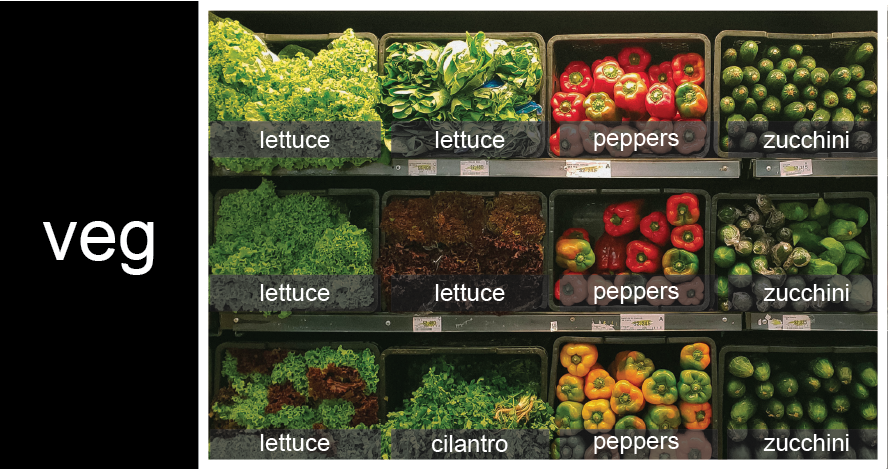
To store the contents of the shelf in a nested list, you write it this way:
PYTHON
veg = [
  ['lettuce', 'lettuce', 'peppers', 'zucchini'],
  ['lettuce', 'lettuce', 'peppers', 'zucchini'],
  ['lettuce', 'cilantro', 'peppers', 'zucchini']
]
Here are some visual examples of how indexing a list of lists
veg works. First, you can reference each row on the shelf
as a separate list. For example, veg[2] represents the
bottom row, which is a list of the baskets in that row.
![veg is now shown as a list of three rows, with veg[0] representing the top row of three baskets, veg[1] representing the second row, and veg[2] representing the bottom row.](../fig/04_groceries_veg0.png)
Index operations using the image would work like this:
OUTPUT
['lettuce', 'cilantro', 'peppers', 'zucchini']OUTPUT
['lettuce', 'lettuce', 'peppers', 'zucchini']To reference a specific basket on a specific shelf, you use two
indexes. The first index represents the row (from top to bottom) and the
second index represents the specific basket (from left to right). For
instance, the cilantro is in the last row, second column,
veg[-1][1].
OUTPUT
'cilantro'![veg is now shown as a two-dimensional grid, with each basket labeled according to its index in the nested list. The first index is the row number and the second index is the basket number, so veg[1][3] represents the basket on the far right side of the second row (basket 4 on row 2): zucchini](../fig/04_groceries_veg00.png)
OUTPUT
'lettuce'OUTPUT
'peppers'There are many ways to change the contents of lists besides assigning new values to individual elements:
OUTPUT
`odds` after adding a value: [1, 3, 5, 7, 11]PYTHON
removed_element = odds.pop(0)
print('odds after removing the first element:', odds)
print('removed_element:', removed_element)
OUTPUT
odds after removing the first element: [3, 5, 7, 11]
removed_element: 1OUTPUT
odds after reversing: [11, 7, 5, 3]While modifying in place, it is useful to remember that Python treats lists in a slightly counter-intuitive way.
As we saw earlier, when we modified the mild_salsa list
item in-place, if we make a list, (attempt to) copy it and then modify
this list, we can cause all sorts of trouble. This also applies to
modifying the list using the above functions:
PYTHON
odds = [3, 5, 7]
primes = odds
primes.append(2)
print('primes:', primes)
print('odds:', odds)
OUTPUT
primes: [3, 5, 7, 2]
odds: [3, 5, 7, 2]
This is because Python stores a list in memory, and then can use
multiple names to refer to the same list. If all we want to do is copy a
(simple) list, we can again use the deepcopy method from
the copy built-in library, so we do not modify a list we
did not mean to:
PYTHON
import copy
odds = [3, 5, 7]
primes = copy.deepcopy(odds)
primes.append(2)
print('primes:', primes)
print('odds:', odds)
OUTPUT
primes: [3, 5, 7, 2]
odds: [3, 5, 7]
Subsets of lists and strings can be accessed by specifying ranges of values in brackets. This is commonly referred to as “slicing” the list/string.
PYTHON
binomial_name = 'Drosophila melanogaster'
group = binomial_name[0:10]
print(f'group: {group}')

species = binomial_name[11:23]
print(f'species: {species}')

# using built-in string methods:
# the split method splits a string into a list wherever a blank space
# occurs (by default)
group,species = binomial_name.split()
# \n is interpreted as the newline character
print(f'group: {group}\nspecies: {species}')

chromosomes = ['X', 'Y', '2', '3', '4']
autosomes = chromosomes[2:5]
print(f'autosomes: {autosomes}')

last = chromosomes[-1]
print('last:', last)
OUTPUT
group: Drosophila
species: melanogaster
group: Drosophila
species: melanogaster
autosomes: ['2', '3', '4']
last: 4Slicing From the End
Use slicing to access only the last four characters of a string or entries of a list.
PYTHON
string_for_slicing = 'Observation date: 02-Feb-2013'
list_for_slicing = [
  ['fluorine', 'F'],
  ['chlorine', 'Cl'],
  ['bromine', 'Br'],
  ['iodine', 'I'],
  ['astatine', 'At'],
]
OUTPUT
'2013'
[['chlorine', 'Cl'], ['bromine', 'Br'], ['iodine', 'I'], ['astatine', 'At']]
Would your solution work regardless of whether you knew beforehand the length of the string or list (e.g. if you wanted to apply the solution to a set of lists of different lengths)? If not, try to change your approach to make it more robust.
Hint: Remember that indices can be negative as well as positive
Non-Contiguous Slices
So far we’ve seen how to use slicing to take single blocks of successive entries from a sequence. But what if we want to take a subset of entries that aren’t next to each other in the sequence?
You can achieve this by providing a third argument to the range within the brackets, called the step size. The example below shows how you can take every third entry in a list:
PYTHON
primes = [2, 3, 5, 7, 11, 13, 17, 19, 23, 29, 31, 37]
subset = primes[0:12:3]
print('subset', subset)
OUTPUT
subset [2, 7, 17, 29]Notice that the slice taken begins with the first entry in the range, followed by entries taken at equally-spaced intervals (the steps) thereafter. If you wanted to begin the subset with the third entry, you would need to specify that as the starting point of the sliced range:
PYTHON
primes = [2, 3, 5, 7, 11, 13, 17, 19, 23, 29, 31, 37]
subset = primes[2:12:3]
print('subset', subset)
OUTPUT
subset [5, 13, 23, 37]Use the step size argument to create a new string that contains only every other character in the string “In an octopus’s garden in the shade”. Start with creating a variable to hold the string:
What slice of beatles will produce the following output
(i.e., the first character, third character, and every other character
through the end of the string)?
OUTPUT
I notpssgre ntesaeIf you want to take a slice from the beginning of a sequence, you can omit the first index in the range:
PYTHON
date = 'Monday 4 January 2016'
day = date[0:6]
print('Using 0 to begin range:', day)
day = date[:6]
print('Omitting beginning index:', day)
OUTPUT
Using 0 to begin range: Monday
Omitting beginning index: Monday
And similarly, you can omit the ending index in the range to take a slice to the very end of the sequence:
PYTHON
# These could all be set on one-line, but "exploding" improves
# readability and commentability
months = [
  'jan',
  'feb',
  'mar',
  'apr',
  'may',
  'jun',
  'jul',
  'aug',
  'sep',
  'oct',
  'nov',
  'dec',
]
sond = months[8:12]
print('With known last position:', sond)
sond = months[8:len(months)]
print('Using len() to get last entry:', sond)
sond = months[8:]
print('Omitting ending index:', sond)
OUTPUT
With known last position: ['sep', 'oct', 'nov', 'dec']
Using len() to get last entry: ['sep', 'oct', 'nov', 'dec']
Omitting ending index: ['sep', 'oct', 'nov', 'dec']Overloading
+ usually means addition, but when used on strings or
lists, it means “concatenate.” Given that, what do you think the
multiplication operator * does on lists? In particular,
what will be the output of the following code?
[2, 4, 6, 8, 10, 2, 4, 6, 8, 10][4, 8, 12, 16, 20][[2, 4, 6, 8, 10], [2, 4, 6, 8, 10]][2, 4, 6, 8, 10, 4, 8, 12, 16, 20]
The technical term for this is operator overloading: a
single operator, like + or *, can do different
things depending on what it’s applied to.
Dictionaries
Dictionaries are the second of two major workhorses in Python codes
for easily collecting multiple values under a single variable name. Like
lists, dictionary values are capable of containing all other objects as
elements, including nested dictionaries or lists. However, unlike lists
— which always use integers starting from 0 elements —
dictionaries allow for arbitrary indices, called
keys, that must simply be immutable. This
means that a dictionary or list cannot be a key, but integers, floats,
complex floats, tuples, sets, and especially strings may be.
We create our first dictionary by explicitly declaring its key-value pairs with colons and comma-separated elements within curly brackets:
PYTHON
squares = {1:1, 2:4, 3:9, 4:16, 'five':'twenty-five'}
print(squares)
print(squares[1], squares[4], squares['five'])
OUTPUT
{1: 1, 2: 4, 3: 9, 4: 16, 'five': 'twenty-five'}}
1 16 twenty-five 100
Once a dictionary is created, new key-value pairs can be appended by associating a new value to a new key:
OUTPUT
{1: 1, 2: 4, 3: 9, 4: 16, 'five': 'twenty-five', 10: 100}Since Python 3.9, two dictionaries may be merged with the
| operator,
OUTPUT
{1: 1, 2: 4, 3: 9, 4: 16, 'five': 'twenty-five', 10: 100, 6: 36, 7: 49}There are two ways to remove a key-value pair:
PYTHON
# del is a built-in statement for deleting workspace objects
del squares['five']
# or
removed_value = squares.pop(10)
Trying to access a dictionary via an undefined key-value pair will
throw a KeyError exception:
OUTPUT
---------------------------------------------------------------------------
KeyError                                  Traceback (most recent call last)
----> 1 print(squares[8])

KeyError: 8
Another common way to create dictionaries involves the constructor
function, dict(), but this will only work for
str-type keys:
PYTHON
periodic_table = dict(
  Hydrogen = 'H',
  Helium   = 'He',
  Lithium  = 'Li',
  Beryllium= 'Be',
  Boron    = 'B',
  Carbon   = 'C',
  Nitrogen = 'N',
  Oxygen   = 'O',
  Fluorine = 'F',
  Neon     = 'Ne',
)
print(periodic_table)
OUTPUT
{'Hydrogen': 'H', 'Helium': 'He', 'Lithium': 'Li', 'Beryllium': 'Be',
'Boron': 'B', ' Carbon': 'C', 'Nitrogen': 'N', 'Oxygen': 'O',
'Fluorine': 'F', 'Neon': 'Ne'}
The advantage of this alternative is that it’s more transparent to
the layperson (dict(...) vs. {...}) and if a
dictionary with pure string keys needs to be created, the lack of quotes
on the key names saves the programmer time.
When the programmer wants to build containers of values with more explicit or meaningful mappings than sequences of natural numbers, dictionaries provide an invaluable data structure. Any time an application accesses multiple lists simultaneously, consider whether a dictionary would improve the readability of your code.
Dictionary operations
Consider the following two dictionaries.
PYTHON
APM_Fall23_grad_courses = {
  501 : 'ODEs',
  503 : 'Analysis',
  505 : 'Linear Algebra',
}
MAT_Fall23_grad_courses = {
  501 : 'Topology',
  512 : 'Combinatorics',
  516 : 'Graph Theory',
}
Determine the outcome of the following code:
What if you swap the operands on either side of the
pipe |?
What would be a better data structure convention to prevent loss of
information after the use of |?
The two dictionaries will be merged into a new dictionary object,
grad_courses, that will contain five key-value pairs. The
collision of the 501 key is resolved by taking the
right-side value. So the key 501 will be set to the value
of Topology. When the operands are swapped, the value is
instead set to ODEs.
A simple fix would have been to make the dictionary keys richer,
i.e., APM501 instead of 501.
Conclusion
The next lesson gets into loops, which we will quickly learn are capable of iterating over the items of a list or dictionary. This rich functionality will guide your non-numeric data structures when programming with Python.
-
[value1, value2, value3, ...]creates a list. -
{key1:value1, key2:value2, ...}creates a dictionary. - Dictionary keys have to be immutable objects, like
ints,floats, but especiallystrs. - Lists and dictionaries values may be any Python object, including themselves (i.e., list of lists or dictionaries of dictionaries).
- Lists are indexed and sliced with square brackets (e.g.,
list[0]andlist[2:9]), in the same way as strings. - Dictionaries are indexed with square brackets too (e.g.,
dict['Neon']). - Lists and dictionaries are mutable (i.e., their values can be changed in place).
- Strings are immutable (i.e., the characters in them cannot be changed).
Content from Repeating Actions with Loops
Last updated on 2024-12-02 | Edit this page
Estimated time: 30 minutes
Overview
Questions
- How can I do the same operations on many different values?
Objectives
- Explain what a
forloop does. - Correctly write
forloops to repeat simple calculations. - Trace changes to a loop variable as the loop runs.
- Trace changes to other variables as they are updated by a
forloop.
Iterating over lists
An example task that we might want to repeat is accessing numbers in a list, which we will do by printing each number on a line of its own.
In Python, a list is basically an ordered collection of elements, and
every element has a unique number associated with it — its index. This
means that we can access elements in a list using their indices. For
example, we can get the first number in the list odds, by
using odds[0]. One way to print each number is to use four
print statements:
OUTPUT
1
3
5
7
This is a terrible approach for three reasons:
Not scalable. Imagine you need to print a list that has \(N\) elements.
Difficult to maintain. If we want to format each printed element with an asterisk or any other character, we would have to change four lines of code. While this might not be a problem for small lists, it would definitely be a problem for longer ones.
Fragile. If we use it with a list that has more elements than what we initially envisioned, it will only display part of the list’s elements. A shorter list, on the other hand, will cause an error because it will be trying to display elements of the list that do not exist.
OUTPUT
1
3
5
ERROR
---------------------------------------------------------------------------
IndexError                                Traceback (most recent call last)
<ipython-input-3-7974b6cdaf14> in <module>()
      3 print(odds[1])
      4 print(odds[2])
----> 5 print(odds[3])

IndexError: list index out of range
Here’s a better approach: a for loop
OUTPUT
1
3
5
7
This is shorter — certainly shorter than something that prints every number in a hundred-number list — and more robust as well:
OUTPUT
1
3
5
7
9
11
The improved version uses a for loop to repeat an operation — in this case, printing — once for each thing in a sequence. The general form of a loop is:
Using the odds example above, the loop might look like this:

where each number (num) in the variable
odds is looped through and printed one number after
another. The other numbers in the diagram denote which loop cycle the
number was printed in (1 being the first loop cycle, and 6 being the
final loop cycle).
We can call the loop
variable anything we like, but there must be a colon at
the end of the line starting the loop, and we must indent anything we
want to run inside the loop. Unlike many other languages,
there is no command to signify the end of the loop body
(e.g. end for); everything indented after the
for statement belongs to the loop.
What’s in a name?
In the example above, the loop variable was given the descriptive
name odd_number. We can choose any name we want for these
loop variables. We might just as easily have chosen the name
banana for the loop variable, as long as we use the same
name when we invoke the variable inside the loop:
OUTPUT
1
3
5
7
9
11
It is a good idea to choose variable names that are meaningful, otherwise it would be more difficult to understand what the loop is doing.
Here’s another loop that repeatedly updates a variable:
PYTHON
length = 0
names = ['Curie', 'Noether', 'Turing']
for value in names:
    length = length + 1
print(f'There are {length} names in the list.')
OUTPUT
There are 3 names in the list.It’s worth tracing the execution of this little program step by step.
Since there are three names in names, the statement on line
4 will be executed three times. The first time around,
length is zero (the value assigned to it on line 1) and
value is Curie. The statement adds 1 to the
old value of length, producing 1, and updates
length to refer to that new value. The next time around,
value is Darwin and length is 1,
so length is updated to be 2. After one more update,
length is 3; since there is nothing left in
names for Python to process, the loop finishes and the
print function on line 5 tells us our final answer. We and
Python know the loop is over by line 5 because of the indenting of the
code block.
Note that a loop variable is a variable that is being used to record progress in a loop. It still exists after the loop is over, and we can re-use variables previously defined as loop variables as well:
PYTHON
name = 'Rosalind'
for name in ['Curie', 'Noether', 'Turing']:
    print(name)
print(f'After the loop, `name` is set to {name}')
OUTPUT
Curie
Noether
Turing
After the loop, `name` is set to Turing
Recall also that finding the length of an object is such a common
operation that Python actually has a built-in function to do it called
len:
OUTPUT
4len is much faster than any function we could write
ourselves, and much easier to read than a two-line loop; it will also
give us the length of many other things that we haven’t met yet, so we
should always use it when we can.
Iterating over ranges
Python has a built-in function called range that
generates a sequence of numbers. range can accept 1, 2, or
3 parameters.
- If one parameter is given,
rangegenerates a sequence of that length, starting at zero and incrementing by 1. For example,range(3)produces the numbers0, 1, 2. - If two parameters are given,
rangestarts at the first and ends just before the second, incrementing by one. For example,range(2, 5)produces2, 3, 4. - If
rangeis given 3 parameters, it starts at the first one, ends just before the second one, and increments by the third one. For example,range(3, 10, 2)produces3, 5, 7, 9.
Summing a list
Write a loop that calculates the sum of elements in a list by adding
each element and printing the final value, so
[124, 402, 36] prints 562
Iterating over strings
In Python, any iterable object may be looped over. This, for example, includes the characters in a string.
The body of the loop is executed 6 times.
Using enumerate to iterate over lists
The built-in function enumerate takes a sequential
container object (e.g., a list) and
generates a new sequence of the same length. Each element of the new
sequence is a pair composed of the index (0, 1, 2,…) and the value from
the original sequence:
PYTHON
odds = [1,3,5,7]
for index, odd in enumerate(odds):
    print(f'list_index={index} :: list_value={odd}')
OUTPUT
list_index=0 :: list_value=1
list_index=1 :: list_value=3
list_index=2 :: list_value=5
list_index=3 :: list_value=7
The code above loops through odds, assigning the index
to index and the value to odd.
Computing the Value of a Polynomial
Suppose you have encoded a polynomial as a list of coefficients in the following way: the first element is the constant term, the second element is the coefficient of the linear term, the third is the coefficient of the quadratic term, where the polynomial is of the form \(ax^0 + bx^1 + cx^2\).
OUTPUT
97Write a loop using enumerate(coefs) which computes the
value y of any polynomial, given x and
coefs.
List comprehensions
Often times we want to quickly generate a container object, like a
list. So far, our only method involves the append internal
method. Suppose we want to generate a list of the first five positive
odd numbers:
PYTHON
# create an empty list
odds = []
# loop over integers \in [0,4], append associated odd to odds list
for i in range(5):
    odds.append(2*i+1)
# enumerate over the odds, which provides two loop variables, the
# incremental count from zero `i` and the associated list value `odd`
for i,odd in enumerate(odds):
    print(f'{i} : {odd}')
OUTPUT
0 : 1
1 : 3
2 : 5
3 : 7
4 : 9
This is such a common task that most high-level languages — and even some low-level ones like Fortran — provide a syntactical sugar for quickly creating the same list, via list comprehension:
OUTPUT
0 : 1
1 : 3
2 : 5
3 : 7
4 : 9
Dictionary comprehension
Similarly, if we wanted to create a dictionary via repetition, we
have the implied method of instantiating an empty object and appending
to it. But there is a nuance when comparing to list iteration:
dictionary objects do not work as expected with the
enumerate method. Instead we must access the
items() sub-method of the dictionary object,
PYTHON
squares = {}
for i in range(5):
    squares[i] = i**2
for key,square in squares.items():
    print(f'The square of {key} is {square}')
OUTPUT
The square of 0 is 0
The square of 1 is 1
The square of 2 is 4
The square of 3 is 9
The square of 4 is 16
A dictionary comprehension makes this all the more syntactically sweet:
PYTHON
squares = {i:i**2 for i in range(5)}
for key,square in squares.items():
    print(f'The square of {key} is {square}')
OUTPUT
The square of 0 is 0
The square of 1 is 1
The square of 2 is 4
The square of 3 is 9
The square of 4 is 16
There are also the submethods of keys() and
values() for times when both pairs are unneeded.
Monitoring loop progress
Often times in scientific computing, the majority of a program’s
execution will occur within a loop. For example, when solving a system
of partial or ordinary differential equations, solvers typically must
iteratively step forward in time. Without periodic reporting or
indication of the loop’s status, it may feel like the program will never
end. (We will see examples of this after the upcoming numpy
and plotting lessons.) But for now it’s important to emphasize the
existence of an extremely convenient external third-party module that
provides rich progress bars for loops, tqdm:
OUTPUT
42%|████████████ | 4233/10000 [00:03<00:04, 1183.17it/s]]- Use
for variable in sequenceto process the elements of a sequence one at a time. - The body of a
forloop must be indented. - Use
len(thing)to determine the length of something that contains other values. - Use
enumerateto obtain loop variables for a sequential object’s indices and values. - List and dictionary comprehensions provide a fast and convent way to initialize those objects.
- Use the
tqdmmodule to create rich progress bars that give a better indication of the loop’s status and provide rough benchmarks.
Content from Conditionals
Last updated on 2024-12-02 | Edit this page
Estimated time: 30 minutes
Overview
Questions
- How can my programs do different things based on data values?
Objectives
- Write conditional statements including
if,elif, andelsebranches. - Correctly evaluate expressions containing
andandor.
In this lesson, we’ll learn how to write code that runs only when certain conditions are true.
Making choices
We can ask Python to take different actions, depending on a
condition, with an if statement:
OUTPUT
not greater
done
The second line of this code uses the keyword if to tell
Python that we want to make a choice. If the test that follows the
if statement is true, the body of the if
(i.e., the set of lines indented underneath it) is executed, and
“greater” is printed. If the test is false, the body of the
else is executed instead, and “not greater” is printed.
Only one or the other is ever executed before continuing on with program
execution to print “done”:

Conditional statements don’t have to include an else. If
there isn’t one, Python simply does nothing if the test is false:
PYTHON
num = 53
print('before conditional...')
if num > 100:
    print(num, 'is greater than 100')
print('...after conditional')
OUTPUT
before conditional...
...after conditional
We can also chain several tests together using elif,
which is short for “else if”. The following Python code uses
elif to print the sign of a number.
PYTHON
num = -3

if num > 0:
    print(num, 'is positive')
elif num == 0:
    print(num, 'is zero')
else:
    print(num, 'is negative')
OUTPUT
-3 is negativeNote that to test for equality we use a double equals sign
== rather than a single equals sign = which is
used to assign values.
Comparing in Python
Along with the > and == operators we
have already used for comparing values in our conditionals, there are a
few more options to know about:
-
>: greater than -
<: less than -
==: equal to -
!=: does not equal -
>=: greater than or equal to -
<=: less than or equal to
We can also combine tests using and and or.
and is only true if both parts are true:
PYTHON
if (1 > 0) and (-1 >= 0):
    print('both parts are true')
else:
    print('at least one part is false')
OUTPUT
at least one part is falsewhile or is true if at least one part is true:
OUTPUT
at least one test is true
True and False
True and False are special words in Python
called booleans, which represent truth values. A statement
such as 1 < 0 returns the value False,
while -1 < 0 returns the value True.
C gets printed because the first two conditions,
4 > 5 and 4 == 5, are not true, but
4 < 5 is true. In this case only one of these conditions
can be true for at a time, but in other scenarios multiple
elif conditions could be met. In these scenarios only the
action associated with the first true elif condition will
occur, starting from the top of the conditional section. 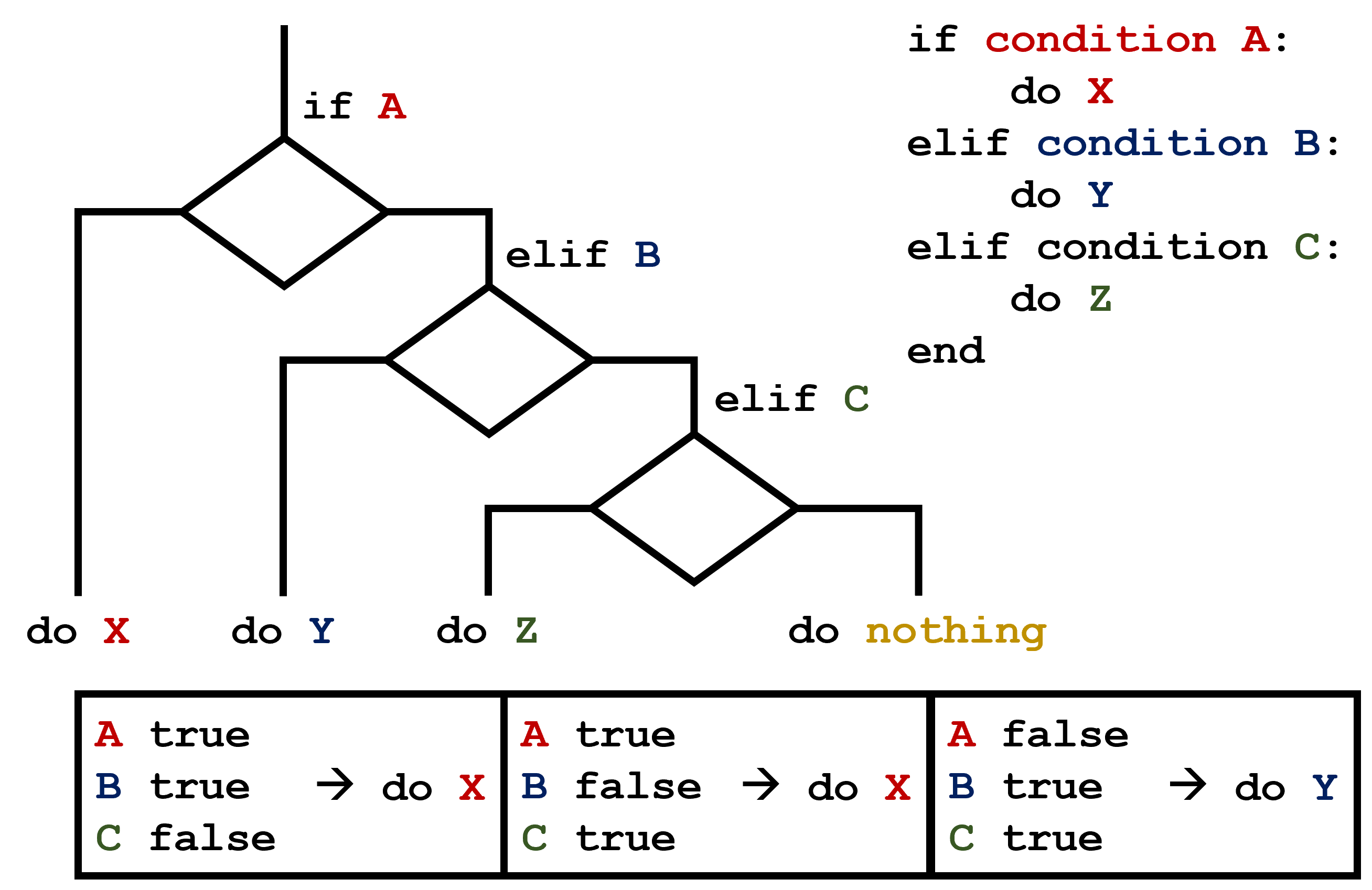 This contrasts with the case of multiple
 if statements,
where every action can occur as long as their condition is met. 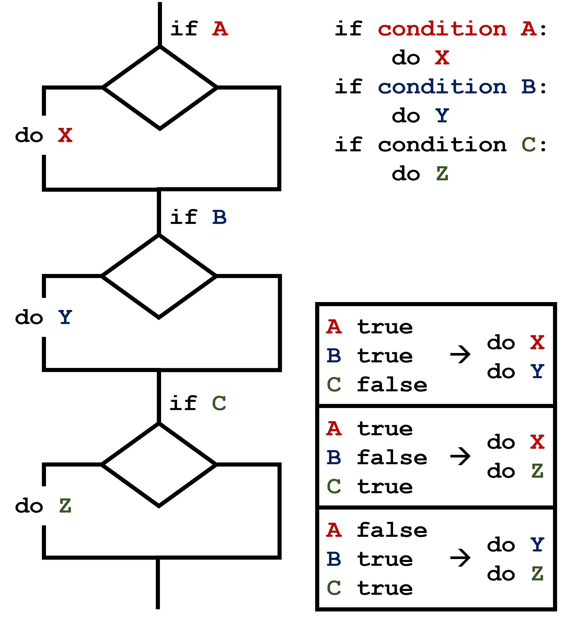
What Is Truth?
True and False booleans are not the only
values in Python that are true and false. In fact, any value
can be used in an if or elif. After reading
and running the code below, explain what the rule is for which values
are considered true and which are considered false.
That’s Not Not What I Meant
Sometimes it is useful to check whether some condition is not true.
The Boolean operator not can do this explicitly. After
reading and running the code below, write some if
statements that use not to test the rule that you
formulated in the previous challenge.
Close Enough
Write some conditions that print True if the variable
a is within 10% of the variable b and
False otherwise. Compare your implementation with your
partner’s: do you get the same answer for all possible pairs of
numbers?
There is a built-in
function abs that returns the absolute value of a
number:
OUTPUT
12In-Place Operators
Python (and most other languages in the C family) provides in-place operators that work like this:
PYTHON
# original value
x = 1
# add one to x, assigning new result back to x
x += 1
# multiply previous value of x by 3, assinging new result back to x
x *= 3
print(x)
OUTPUT
6Write some code that sums the positive and negative numbers in a list separately, using in-place operators. Do you think the result is more or less readable than writing the same without in-place operators?
PYTHON
positive_sum = 0
negative_sum = 0
test_list = [3, 4, 6, 1, -1, -5, 0, 7, -8]
for num in test_list:
    if num > 0:
        positive_sum += num
    elif num == 0:
        pass
    else:
        negative_sum += num
print(positive_sum, negative_sum)
Here pass means “don’t do anything”. In this particular
case, it’s not actually needed, since if num == 0 neither
sum needs to change, but it illustrates the use of elif and
pass.
Sorting a List Into Buckets
In our data folder, large data sets are stored in files
whose names start with “inflammation-” and small data sets — in files
whose names start with “small-”. We also have some other files that we
do not care about at this point. We’d like to break all these files into
three lists called large_files, small_files,
and other_files, respectively.
Add code to the template below to do this. Note that the string
method startswith
returns True if and only if the string it is called on
starts with the string passed as an argument, that is:
OUTPUT
TrueBut
OUTPUT
FalseUse the following Python code as your starting point:
PYTHON
filenames = [
  'inflammation-01.csv',
  'myscript.py',
  'inflammation-02.csv',
  'small-01.csv',
  'small-02.csv',
]
large_files = []
small_files = []
other_files = []
Your solution should:
- loop over the names of the files
- figure out which group each filename belongs in
- append the filename to that list
In the end the three lists should be:
PYTHON
for filename in filenames:
    if filename.startswith('inflammation-'):
        large_files.append(filename)
    elif filename.startswith('small-'):
        small_files.append(filename)
    else:
        other_files.append(filename)

print('large_files:', large_files)
print('small_files:', small_files)
print('other_files:', other_files)Counting Vowels
- Write a loop that counts the number of vowels in a character string.
- Test it on a few individual words and full sentences.
- Once you are done, compare your solution to your neighbor’s. Did you make the same decisions about how to handle the letter ‘y’ (which some people think is a vowel, and some do not)?
- Use
if conditionto start a conditional statement,elif conditionto provide additional tests, andelseto provide a default. - The bodies of the branches of conditional statements must be indented.
- Use
==to test for equality. -
X and Yis only true if bothXandYare true. -
X or Yis true if eitherXorY, or both, are true. - Zero, the empty string, and the empty list are considered false; all other numbers, strings, and lists are considered true.
-
TrueandFalserepresent truth values.
Content from Numeric Python (NumPy)
Last updated on 2024-12-05 | Edit this page
Estimated time: 60 minutes
Overview
Questions
- How can I process tabular data files in Python?
Objectives
- Explain what a library is and what libraries are used for.
- Import a Python library and use the functions it contains.
- Read tabular data from a file into a program.
- Select individual values and subsections from data.
- Perform operations on arrays of data.
\(\newcommand{\coloneq}{\mathrel{≔}}\) \(\def\doubleunderline#1{\underline{\underline{#1}}}\) \(\def\tripleunderline#1{\underline{\doubleunderline{#1}}}\) \(\def\tprod{{\small \otimes}}\) \(\def\tensor#1{{\bf #1}}\) \(\def\mat#1{{\bf #1}}\) \(\renewcommand{\vec}[1]{{\bf #1}}\) \(\def\e{\vec{e}}\)
Words are useful, but what’s more useful are the sentences and stories we build with them. Similarly, while a lot of powerful, general tools are built into Python, specialized tools built up from these basic units live in libraries that can be called upon when needed.
The ndarray
The base work-horse of the NumPy framework is the
ndarray object. This object provides a performant container
for tensor algebra. Its performance, capabilities, base coverage, and
syntactical flavor are all based on the default array type from MATLAB,
but arguably provides greater flexibility for the programmer, especially
for third-order or larger tensors.
For those familiar with MATLAB, many syntactical features and operations will seem familiar, but there are subtle differences that may be awkward at first. For a full reference, see the official docs, NumPy for MATLAB users, which provides a Rosetta-Stone-like guide for MATLAB users.
The very first thing to do in Python to work with NumPy is to import the external library:
This line of code imports the external library into the workspace,
renaming it by common convention to np. The
as np is a shorthand that would have been equivalent to a
second line of code assigning the name np=numpy. For the
rest of this lesson, we will assume that NumPy has been
imported into the workspace as np. This only
has to be done once per Python invocation. Typically, it will be done at
the top of a Python script (in the header), or in the very first cell of
a Jupyter notebook.
To actually use the library — i.e., access the classes and methods
within it — we have to write np. and then the target
code.
OUTPUT
[0 1 2 3 4]
 `a` is of type: <class 'numpy.ndarray'>
 and `a[0]` type: <class 'numpy.int64'>
The code above prints the result of using the
numpy.arange method, which is similar to the built-in
range method, but in this instance instead generates a
one-dimensional ndarray object with the first five
non-negative integers (recall, Python is zero-indexed). Also, the
elements of the generated ndarray, a, are not
“vanilla” Python int objects. Instead they are 64-bit
integer objects provided by the NumPy library. This is an implicit hint
that we are using Python as a medium for all future computations: Python
is slow so we use it as a convienent interface
with fast NumPy to set up the data structures and communicate logical
instructions for data transformations.
Note that numpy.arange is an
overloaded function, meaning that we can pass
a floating-point argument to generate the appropriate NumPy
ndarray of numpy.float64 values very
easily.
OUTPUT
[0. 1. 2. 3. 4.]
 `x` is of type: <class 'numpy.ndarray'>
 and `x[0]` type: <class 'numpy.float64'>
This is a valid use of the numpy.arange method, but
typically we will want to only generate ranges of
numpy.int64 with the method. The rest of the materials will
only use the arange method for generating integer
ndarrays.
Unlike the built-in list, the NumPy ndarray
automatically broadcasts scalar arithmetic to
the elements of the ndarray:
OUTPUT
1+a: [1 2 3 4 5]
2*a: [0 2 4 6 8]
For MATLAB users,
np.arange(<start>,<excluded end>,<stride>)
provides functionality like the colon operator,
<start>:<stride>:<included end>. Thus, we
may generate an ndarray of odd numbers without list
comprehension, improving performance as a perk,
PYTHON
# benchmark generating the first ten-million odds with vanilla Python
# NOTE: `%timeit` is a "Jupyter Magic," a Jupyter macro, not Python!
%timeit odd_list = [2*k+1 for k in range(10**7)]
%timeit odd_list2 = [k for k in range(1,2*10**7,2)]
%timeit odd_list3 = list(range(1,2*10**7,2))
OUTPUT
393 ms ± 884 µs per loop (mean ± std. dev. of 7 runs, 1 loop each)
198 ms ± 544 µs per loop (mean ± std. dev. of 7 runs, 10 loops each)
148 ms ± 207 µs per loop (mean ± std. dev. of 7 runs, 10 loops each)
PYTHON
# benchmark generating the first ten-million odds with NumPy
%timeit odd_array = 2*np.arange(10**7)+1
# Even less Python and more NumPy:
%timeit odd_array2 = np.arange(1,2*10**7,2)
OUTPUT
13 ms ± 550 µs per loop (mean ± std. dev. of 7 runs, 100 loops each)
8 ms ± 90 µs per loop (mean ± std. dev. of 7 runs, 100 loops each)
Vanilla Python is, at best and worst, nearly 20–50 times slower than NumPy! Why is this? It may help to spell out the operations involved.
Vanilla Python
In this approach, Python is asked to do ten-million product and sum
operations (twenty-million actions), and store the results in a generic,
unoptimized list object. The second attempt redundantly
converts the generated iterates of range(1,2*10**7,2) to a
list, improving performance by a factor of two. The final attempt
removes the redundant list comprehension.
First NumPy approach
In this solution, odd_array = 2*np.arange(10**7)+1,
NumPy is asked to generate a list of the first ten-million non-negative
integers, which is done in a performant C library with the updated
memory accessible from Python’s workspace. Then NumPy is told — through
broadcasting — to multiply every element by two and add one. It’s still
twenty-million actions, but the difference is that Python is only
involved up to three times; the rest is done in an expertly written
backend library which is nearly 30 times faster than the comparable
approach in vanilla Python.
Naive matrix multiplication
This next example would have been counter productive to introduce prior to NumPy, as it is an exhausting exercise to even generate two-dimensional lists in vanilla Python. However, it’s much simpler with NumPy. For instance, to generate a four-by-four of uniformly random numbers in \((0,1)\):
OUTPUT
[[0.95781959 0.9915284  0.58248825 0.41600528]
 [0.77493045 0.67522185 0.00530085 0.2539285 ]
 [0.53248467 0.75761823 0.69219508 0.58811258]
 [0.59892653 0.77743011 0.95975933 0.71425297]]
Or we would have to use the standard random library,
which encourages bad habits (technique with Python lists and
random that should not be practiced, although nested list
comprehension has its place in the toolbox):
PYTHON
import random
A = [ [random.random() for column in range(4)] for row in range(4) ]
for row in A: print(row)
OUTPUT
[0.6818582562400426, 0.6868889674612016, 0.34483486515037653, 0.9638090861458387]
[0.24086075915520622, 0.07221778821332858, 0.43624157264612706, 0.7935877715986276]
[0.6585256801337919, 0.2631377880223672, 0.9586513851146543, 0.9070537970347129]
[0.1566693962998439, 0.8860807403362514, 0.039423876906426014, 0.44815646838680734]
We will write a few functions to do matrix multiplication with vanilla Python.
PYTHON
def vanilla_dot_product(u,v):
    running_sum = 0
    for i in range(len(u)):
        running_sum += u[i]*v[i]
    return running_sum
def vanilla_matrix_vector_product(A,x):
    y = [ vanilla_dot_product(a,x) for a in A ]
    return y
def vanilla_matrix_tranpose(A):
    # `*A` passes the first-elements of `A` --- the rows --- to zip as
    # arguments, as if we wrote every row of `A` explicitly.
    # `zip` is a built-in function that iteratively combines the first
    # elements of its arguments, allowing us to iterate over the cols of
    # `A`.
    # `map` is a built-in function that shortcuts a for loop: we are
    # mapping every column of `A` to the `list` class, converting the
    # immutable tuples to lists.
    # The final `list` ensures that `A_Transposed` is a two-dimensional
    # container of "column vectors."
    A_Tranposed = list(map(list,zip(*A)))
    return A_Tranposed
def vanilla_matrix_matrix_product(A,B):
    # `*B` passes the first-elements of `B` --- the rows --- to zip as
    # arguments, as if we wrote every row of `B` explicitly.
    # `zip` is a built-in function that iteratively combines the first
    # elements of its arguments, allowing us to iterate over the cols of
    # `B`.
    CT = [ vanilla_matrix_vector_product(A,b_col) for b_col in zip(*B) ]
    C  = vanilla_matrix_tranpose(CT)
    return C
PYTHON
# originally 1000x1000, but list method takes way too long
A,B = np.random.rand(2,100,100)
AL,BL = A.tolist(),B.tolist()
%timeit CL = vanilla_matrix_matrix_product(AL,BL)
# A@B implicitly calls LAPACK dgemm and parallelizes if multiple cores
%timeit C = A@B
# Validate accuracy of custom matrix-matrix product
CL = vanilla_matrix_matrix_product(AL,BL)
C  = A@B
# compute elementwise error matrix
elementwise_error = C - np.array(CL)
# print out the Frobenius norm of the error matrix
print(f'Fro. norm: {np.linalg.norm(elementwise_error)}')
# Another way to check
print(f'Are all elements close? {np.all(np.isclose(C,np.array(CL)))}')
OUTPUT
22.5 ms ± 58.7 µs per loop (mean ± std. dev. of 7 runs, 10 loops each)
303 µs ± 15.5 µs per loop (mean ± std. dev. of 7 runs, 1,000 loops each)
Fro. norm: 2.3464053421603193e-13
Are all elements close? True
The simpler matrix-matrix product provided by NumPy, by just using
the @ operator for the two matrices, is nearly 65 times
faster than the vanilla approach, and will automatically use multiple
cores for us.
Approximating derivatives
The second-order, central finite difference stencil, \[\dfrac{u(x_{i+1})-u(x_{i-1})}{2\Delta x},\] where \(\Delta x=x_1-x_0\) is the uniform spatial step, approximates the first derivative of a function \(u\) at a point \(x_i\). Let \(u(x)=\sin(x)\) for \(x\in[0,2\pi)\) and discretize the domain such that \(x_i = 2\pi i/N\) for \(i=0,...,N\). Use NumPy matrix multiplication to compute the first derivative of \(u\) with \(N=10^k\) for \(k=1,...,4\), by constructing the appropriate dense operator \(D\) for the stencil. Using a 2-norm, how does the error change with \(\Delta x\)?
Extra Credit: since the stencil is very sparse, how could we improve the performance of the code and go to larger \(N\)? What is the largest \(N\) we could go to, and why?
The discretization of the domain together with the periodicity of \(u\) and the second-order stencil induces a set of linear equations, \[D_{ij}u_j \approx u_j',\] \[ \dfrac{1}{2\Delta x} \begin{bmatrix} 0 & 1 & 0 & ... & 0 & -1 \\ -1 & 0 & 1 & 0 & & 0 \\ 0 & -1 & 0 & \ddots &\ddots& \vdots\\ \vdots & 0 & \ddots & \ddots & 1 & 0 \\ 0 & & \ddots & -1 & 0 & 1 \\ 1 & 0 & ... & 0 & -1 & 0 \\ \end{bmatrix} \begin{bmatrix} u(x_0) \\ u(x_1) \\ \vdots \\ u(x_{N-3}) \\ u(x_{N-2}) \\ u(x_{N-1}) \\ \end{bmatrix} \approx \begin{bmatrix} u'(x_0) \\ u'(x_1) \\ \vdots \\ u'(x_{N-3}) \\ u'(x_{N-2}) \\ u'(x_{N-1}) \\ \end{bmatrix}, \] where \(D\in\mathbb{R}^{N\times N}\).
The following code defines a function, challenge, which
takes an input \(N\) and computes the
relative error. It also plots the degree of error on a log.-log. scale,
demonstrating that the stencil’s truncation error converges to the
analytical solution quadratically with the step size, \(\Delta x\).
PYTHON
import numpy as np
import matplotlib.pyplot as plt
def challenge(N):
    # N+1 is important here, because definition of x
    x = np.linspace(0,2*np.pi,N+1)[:-1]
    dx= x[1]-x[0]
    u = np.sin(x)
    # put 1 and -1 on super- and sub-diagonal, respectively
    D = np.diag(np.ones(N-1),1)-np.diag(np.ones(N-1),-1)
    # circulant derivative operator (periodicity)
    D[0,-1] =-1
    D[-1,0] = 1
    D /= 2*dx
    # compute derivative
    du= D@u
    # exact result
    ex= np.cos(x)
    rel_err = np.linalg.norm(ex-du)/np.linalg.norm(ex)
    return rel_err

Ns = 10**np.arange(1,5)
rel_errs = np.array([challenge(N) for N in Ns])
dxs = 2*np.pi / Ns
plt.loglog(dxs,rel_errs,'ro-',linewidth=2,label='Relative Error')
c = np.polyfit(np.log(dxs),np.log(rel_errs),1)
h = np.logspace(-4,0,41)
E = np.exp(c[1])*h**c[0]
plt.loglog(h,E,'k-',linewidth=3,zorder=-1,label='Algebraic Fit')
plt.legend()
print(f'Relative error is second order in ∆x: {c[0]:.5f}')
OUTPUT
Relative error is second order in ∆x: 1.99742
Discussion
The above approach worked well for \(N\) up to \(10^4\). What would happen in \(N\) were increased much further for the same system? The size of \(D\) grows like \(N^2\), so very quickly we’ll run out of fast CPU memory, called “cache,” and likely run out of RAM too, causing out-of-memory errors.
The stencil in the challenge results in an extremely sparse operator representation for \(D\). Thus, using a dense representation is extremely inefficient, regardless of the performant backend. A better solution code then could have
- used sparse matrices instead of a dense one,
- used index slicing to represent the operations,
- or probably the fastest: used the
np.rollinstead to account for the periodicity.
Demonstrating this last point:
du = (np.roll(u,-1)-np.roll(u,+1))/(2*dx) allows for a much
faster approximation of order \(N\)
instead of \(N^2\).
However, for \(N\) beyond \(10^6\), the error will begin to increase as rounding errors begin to dominate the total error of the approximation.
Attributes of ndarray instances
Jupyter Tips and Tricks
To see all the possible methods and attributes under a workspace
name, like a as defined by
a=np.linspace(0,1,5), use the Tab key after
typing a dot. I.e., typing a+.+Tab will
show a context menu of all possible sub-names to complete for that
object, a.
NumPy’s ndarray class provides its instances with a
variety of rich methods. These methods allow for syntactically sweet
data transformation. We highlight a few of the common methods below.
PYTHON
# generate an `ndarray` over [0,1] with 5 points with uniform spacing,
# such that $x_k=a+k(b-a)/(N-1)$ for $k\in[0,N)\subset\mathbb{Z}$.
a,b,N = 0,1,5
x = np.linspace(a,b,N)
print(f'`x`: {x}\n`x*x`: {x*x}\n`x@x`: {x@x}')
# print a horizontal rule 72-characters long with " x " centered
print(f'{" x ":=^72}')
# summary characteristics for x:
x_min, x_mean, x_max, x_std = x.min(), x.mean(), x.max(), x.std()
print(f'min: {x_min}\nmean: {x_mean}\nmax: {x_max}\nstandard dev.: {x_std}')
x_sum, x_shape, x_transpose = x.sum(), x.shape, x.T
print(f'sum: {x_sum}\nshape: {x_shape}\ntranspose: {x_transpose}')
OUTPUT
`x`: [0.   0.25 0.5  0.75 1.  ]
`x*x`: [0.     0.0625 0.25   0.5625 1.    ]
`x@x`: 1.875
================================== x ===================================
min: 0.0
mean: 0.5
max: 1.0
standard dev.: 0.3535533905932738
sum: 2.5
shape: (5,)
transpose: [0.   0.25 0.5  0.75 1.  ]
Note that these object methods are also functions at NumPy’s root.
For instance, instead of x.min() we could have equivalently
run np.min(x). One reason to do the latter instead of the
former is if we are potentially mixing object types as inputs —
np.min(L) will work when L is a list object,
but then L.min() is undefined. For new and expert users, a
good practice is to use the object’s method calls (x.min())
as it is faster to write and encourages the use of performant
ndarray objects over lists for numerical data.
However, not everything is defined as a method call. For instance,
the median must be computed with np.median. Additionally,
the convenience attribute .T is not a method call, but an
attribute, which returns a view of the
ndarray transposed. Note from the example that
x is truly one-dimensional with five elements and thus
x is equivalent to x.T. We did not have to
worry about the formal linear algebra rules for computing the squared
2-norm of x with x@x — NumPy was able to infer
that we meant to compute the inner product without adding a redundant
second dimension — or axis — to
x.
Linear algebra with NumPy
In this section, we will use some tensor algebra to make the operations more clear, as well as to introduce Einstein summation notation, which will allow us to use a very powerful NumPy tool later.
In tensor algebra, tensors are represented with linear combinations of basis tensors. For instance, for a simple three-dimensional vector, \(\vec{u}\), and a set of Euclidean unit vectors, \(\e_k\),
\[ \vec{u} = \begin{bmatrix}u_1\\u_2\\u_3\end{bmatrix} = u_1 \begin{bmatrix}1\\0\\0\end{bmatrix} + u_2 \begin{bmatrix}0\\1\\0\end{bmatrix} + u_3 \begin{bmatrix}0\\0\\1\end{bmatrix} = u_1 \e_1 + u_2 \e_2 + u_3 \e_3 = \sum_{k=1}^3 u_k \e_k. \]
The Cartesian outer products of Euclidean unit vectors form a natural basis for representing matrices:
\[ \mat{A} = \begin{bmatrix}A_{11}&A_{12}\\A_{21}&A_{22}\\\end{bmatrix} = A_{11} \begin{bmatrix}1&0\\0&0\\\end{bmatrix} + A_{12} \begin{bmatrix}0&1\\0&0\\\end{bmatrix} + A_{21} \begin{bmatrix}0&0\\1&0\\\end{bmatrix} + A_{22} \begin{bmatrix}0&0\\0&1\\\end{bmatrix} \\ = \sum_{j=1}^2\sum_{k=1}^2 A_{jk} \e_j \e_k^T \\ = \sum_{j=1}^2\sum_{k=1}^2 A_{jk} \e_j \tprod \e_k. \]
The notation \(\tprod\) refers to the tensor product that becomes necessary for representing higher-order tensors.
Tensor-tensor calculations then involve carrying out products of sums. For instance, an inner product of two \(\mathbb{R}^2\) vectors:
\[ \vec{u}^T\vec{v} = \left( \sum_{j=1}^2 u_j\e_j \right)^T \sum_{k=1}^2 v_k\vec{e_k} \\ = u_1 v_1 \e_1^T\e_1 + u_1 v_2 \e_1^T\e_2 + u_2 v_1 \e_2^T\e_1 + u_2 v_2 \e_2^T\e_2 \\ = \sum_{j=1}^2\sum_{k=1}^2 u_j v_k\e_j^T\e_k = \sum_{j=1}^2\sum_{k=1}^2 u_j v_k \delta_{jk} = \sum_{j=1}^2 u_j v_j = u_1 v_1 + u_2 v_2, \]
where \(\delta_{jk}\) is the Kronecker delta, which is zero unless \(j=k\), in which case it’s one [thanks to using a(n) (orthonormal) basis].
Einstein Summation Notation
Einstein summation notation is a more compact representation of tensor algebra, that simply drops the summation symbols. Continuing from the matrix example above, \(\mat{A}= A_{jk}\e_j\tprod \e_k\).
The inner product example also reduces to \(\vec{u}\cdot\vec{v}=u_j v_k \e_j\cdot\e_k = u_j v_j\).
D.1.1: One-dimensional ndarray operations
For this sub-section, define the following one-dimensional NumPy
ndarrays and variables:
\[ \texttt{N} \coloneq 5, \\ \textrm{Let: } k\in[0,N)\subset\mathbb{Z}, \\ \texttt{x} \coloneq \vec{x} = \frac{k}{N-1} \e_k, \\ \texttt{a} \coloneq \vec{a} = k \e_k. \]
OUTPUT
x: [0.   0.25 0.5  0.75 1.  ]
a: [0 1 2 3 4]
D.1.1.a elementwise operations
\[\texttt{x+a}\coloneq\vec{x}+\vec{a}= (x_i+a_i) \e_i\]
\[\texttt{x*a}\coloneq\vec{x}\odot\vec{a}= x_i a_i \e_i\]
OUTPUT
x+a: [0.   1.25 2.5  3.75 5.  ]
x*a: [0. 0.25 1. 2.25 4. ]D.1.1.c outer products
\[ \texttt{np.outer(x,a)} \coloneq \vec{x}\tprod\vec{a} =x_i a_j \e_i\tprod\e_j \]
\[ \texttt{np.add.outer(x,a)} \coloneq \vec{x}\tprod\vec{1}+\vec{1}\tprod\vec{a} = (x_i + a_j)\,\, \e_i\tprod\e_j, \]
where \(\vec{1}\) is a vector of all ones.
PYTHON
print(f'vector outer(x,a): (x_i*a_j)e_i e_j\n{np.outer(x,a)}\n')
print(f'addition outer(x,a): (x_i+a_j)e_i e_j\n{np.add.outer(x,a)}\n')
OUTPUT
vector outer(x,a): (x_i*a_j) e_i e_j
[[0.   0.   0.   0.   0.  ]
 [0.   0.25 0.5  0.75 1.  ]
 [0.   0.5  1.   1.5  2.  ]
 [0.   0.75 1.5  2.25 3.  ]
 [0.   1.   2.   3.   4.  ]]

addition outer(x,a): (x_i+a_j) e_i e_j
[[0.   1.   2.   3.   4.  ]
 [0.25 1.25 2.25 3.25 4.25]
 [0.5  1.5  2.5  3.5  4.5 ]
 [0.75 1.75 2.75 3.75 4.75]
 [1.   2.   3.   4.   5.  ]]
D.2.1 Matrix-vector operations
For this sub-section, define the following one- and two-dimensional
NumPy ndarrays and variables:
\[ \texttt{N} \coloneq N=4, \\ \textrm{Let: } k\in[0,N^2)\subset\mathbb{Z}, \quad \mu=\Bigl\lfloor \frac{k}{N}\Bigr\rfloor, \quad \nu= k \bmod N \\ \texttt{A} \coloneq \mat{A} = k^2\,\, \e_\mu \tprod \e_\nu. \\ \textrm{Let: } j\in[0,N)\subset\mathbb{Z}, \\ \texttt{x} \coloneq \vec{x} = (j+1)\,\,\e_j. \]
OUTPUT
A:
 [[  0   1   4   9]
 [ 16  25  36  49]
 [ 64  81 100 121]
 [144 169 196 225]]

x: [1 2 3 4]
D.2.1.a Elementwise
Let \(i,j,k\in[0,N)\subset\mathbb{Z}\).
\[ \texttt{A+x} \coloneq \mat{A} + (\vec{1}\tprod \vec{x}) = (A_{ij}+x_j)\,\e_i\tprod\e_j \]
\[ \texttt{A*x} \coloneq \mat{A} \odot (\vec{1}\tprod \vec{x}) = (A_{ij} x_j)\,\e_i\tprod\e_j \]
OUTPUT
ELEMENTWISE BROADCASTING
        A+x
[[  1   3   7  13]
 [ 17  27  39  53]
 [ 65  83 103 125]
 [145 171 199 229]]

        A*x
[[  0   2  12  36]
 [ 16  50 108 196]
 [ 64 162 300 484]
 [144 338 588 900]]
D.2.1.b Matrix-vector operations
Let \(i,j\in[0,N)\subset\mathbb{Z}\).
\[ \texttt{x@A} \coloneq \vec{x}^T \mat{A} = A_{ij} x_i \e_j^T \]
\[ \texttt{A@x} \coloneq \mat{A} \vec{x} = A_{ij} x_j \e_i \]
OUTPUT
x@A
[ 800  970 1160 1370]

A@x
[  50  370 1010 1970]
D.2.1.c Solving \(\mat{A}\vec{x}=\vec{b}\)
Let \(i,j\in[0,N)\subset\mathbb{Z}\) and let \(\vec{b} = \mat{A}\vec{x}\). Then \(\vec{x}=A^{-1}_{ij}b_j\e_i\).
D.2.1.c.i Matrix inversion (bad)
PYTHON
b = A@x
A_inverse = np.linalg.inv(A)
x_approx  = A_inverse@b
print('Rel. Err.: ',np.linalg.norm(x_approx-x)/np.linalg.norm(x))
OUTPUT
Rel. Err.: 2.294921930407801D.2.1.c.ii Implicit solve (good)
PYTHON
b = A@x
x_approx  = np.linalg.solve(A,b)
print('Rel. Err.: ',np.linalg.norm(x_approx-x)/np.linalg.norm(x))
OUTPUT
Rel. Err.: 0.012225D.2.1.c.iii PLU solve (good, equivalent to previous)
PYTHON
import scipy
b = A@x
LU_and_pivots = scipy.linalg.lu_factor(A)
x_approx  = scipy.linalg.lu_solve(LU_and_pivots,b)
print('Rel. Err.: ',np.linalg.norm(x_approx-x)/np.linalg.norm(x))
OUTPUT
Rel. Err.: 0.012225D.2.1.c.iv Eig solve (worse)
PYTHON
b = A@x
evals,evecs = np.linalg.eig(A)
x_approx = evecs @ (np.linalg.solve(evecs,b)/evals)
print('Rel. Err.: ',np.linalg.norm(x_approx-x)/np.linalg.norm(x))
OUTPUT
Rel. Err.: 16.3456D.2.2 Matrix-matrix operations
For this sub-section, define the following two-dimensional NumPy
ndarrays and variables:
\[ \texttt{N} \coloneq N=2, \\ \textrm{Let: } k\in[0,N^2)\subset\mathbb{Z}, \quad \mu=\Bigl\lfloor \frac{k}{N}\Bigr\rfloor, \quad \nu= k \bmod N \\ \texttt{A} \coloneq \mat{A} = k^2\,\, \e_\mu \tprod \e_\nu \\ \texttt{B} \coloneq \mat{B} = k\,\, \e_\mu \tprod \e_\nu \]
PYTHON
N = 2
A = np.arange(N**2).reshape((N,N))**2
B = np.arange(N**2).reshape((N,N))
print(f'A:\n {A}\n\nB:\n {B}')
OUTPUT
A:
 [[0 1]
 [4 9]]

B:
 [[0 1]
 [2 3]]
D.2.2.a elementwise
Let \(i,j\in[0,N)\subset\mathbb{Z}\).
\[ \texttt{A+B} \coloneq \mat{A} + \mat{B} = (A_{ij} + B_{ij}) \,\, \e_i\tprod\e_j \]
\[ \texttt{A*B} \coloneq \mat{A} \odot \mat{B} = A_{ij} B_{ij} \,\, \e_i\tprod\e_j \]
OUTPUT
ELEMENTWISE BROADCASTING
   A+B
[[ 0  2]
 [ 6 12]]

   A*B
[[ 0  1]
[ 8 27]]Using ndarray built-in methods
Basic signal processing
Loading data into Python
To begin processing the clinical trial inflammation data, we need to load it into Python. We can do that using a library called NumPy, which stands for Numerical Python. In general, you should use this library when you want to do fancy things with lots of numbers, especially if you have matrices or arrays. To tell Python that we’d like to start using NumPy, we need to import it:
Importing a library is like getting a piece of lab equipment out of a storage locker and setting it up on the bench. Libraries provide additional functionality to the basic Python package, much like a new piece of equipment adds functionality to a lab space. Just like in the lab, importing too many libraries can sometimes complicate and slow down your programs - so we only import what we need for each program.
Once we’ve imported the library, we can ask the library to read our data file for us:
OUTPUT
array([[ 0.,  0.,  1., ...,  3.,  0.,  0.],
       [ 0.,  1.,  2., ...,  1.,  0.,  1.],
       [ 0.,  1.,  1., ...,  2.,  1.,  1.],
       ...,
       [ 0.,  1.,  1., ...,  1.,  1.,  1.],
       [ 0.,  0.,  0., ...,  0.,  2.,  0.],
       [ 0.,  0.,  1., ...,  1.,  1.,  0.]])
The expression numpy.loadtxt(...) is a function call that asks Python
to run the function
loadtxt which belongs to the numpy library.
The dot notation in Python is used most of all as an object
attribute/property specifier or for invoking its method.
object.property will give you the object.property value,
object_name.method() will invoke on object_name method.
As an example, John Smith is the John that belongs to the Smith
family. We could use the dot notation to write his name
smith.john, just as loadtxt is a function that
belongs to the numpy library.
numpy.loadtxt has two parameters: the name of the file we
want to read and the delimiter
that separates values on a line. These both need to be character strings
(or strings for short), so we put
them in quotes.
Since we haven’t told it to do anything else with the function’s
output, the notebook displays it.
In this case, that output is the data we just loaded. By default, only a
few rows and columns are shown (with ... to omit elements
when displaying big arrays). Note that, to save space when displaying
NumPy arrays, Python does not show us trailing zeros, so
1.0 becomes 1..
Our call to numpy.loadtxt read our file but didn’t save
the data in memory. To do that, we need to assign the array to a
variable. In a similar manner to how we assign a single value to a
variable, we can also assign an array of values to a variable using the
same syntax. Let’s re-run numpy.loadtxt and save the
returned data:
This statement doesn’t produce any output because we’ve assigned the
output to the variable data. If we want to check that the
data have been loaded, we can print the variable’s value:
OUTPUT
[[ 0.  0.  1. ...,  3.  0.  0.]
 [ 0.  1.  2. ...,  1.  0.  1.]
 [ 0.  1.  1. ...,  2.  1.  1.]
 ...,
 [ 0.  1.  1. ...,  1.  1.  1.]
 [ 0.  0.  0. ...,  0.  2.  0.]
 [ 0.  0.  1. ...,  1.  1.  0.]]
Now that the data are in memory, we can manipulate them. First, let’s
ask what type of thing
data refers to:
OUTPUT
<class 'numpy.ndarray'>The output tells us that data currently refers to an
N-dimensional array, the functionality for which is provided by the
NumPy library. These data correspond to arthritis patients’
inflammation. The rows are the individual patients, and the columns are
their daily inflammation measurements.
Data Type
A NumPy array contains one or more elements of the same type. The
type function will only tell you that a variable is a NumPy
array but won’t tell you the type of thing inside the array. We can find
out the type of the data contained in the NumPy array.
OUTPUT
float64This tells us that the NumPy array’s elements are floating-point numbers.
With the following command, we can see the array’s shape:
OUTPUT
(60, 40)The output tells us that the data array variable
contains 60 rows and 40 columns. When we created the variable
data to store our arthritis data, we did not only create
the array; we also created information about the array, called members or attributes. This extra
information describes data in the same way an adjective
describes a noun. data.shape is an attribute of
data which describes the dimensions of data.
We use the same dotted notation for the attributes of variables that we
use for the functions in libraries because they have the same
part-and-whole relationship.
If we want to get a single number from the array, we must provide an index in square brackets after the variable name, just as we do in math when referring to an element of a matrix. Our inflammation data has two dimensions, so we will need to use two indices to refer to one specific value:
OUTPUT
first value in data: 0.0OUTPUT
middle value in data: 16.0The expression data[29, 19] accesses the element at row
30, column 20. While this expression may not surprise you,
data[0, 0] might. Programming languages like Fortran,
MATLAB and R start counting at 1 because that’s what human beings have
done for thousands of years. Languages in the C family (including C++,
Java, Perl, and Python) count from 0 because it represents an offset
from the first value in the array (the second value is offset by one
index from the first value). This is closer to the way that computers
represent arrays (if you are interested in the historical reasons behind
counting indices from zero, you can read Mike
Hoye’s blog post). As a result, if we have an M×N array in Python,
its indices go from 0 to M-1 on the first axis and 0 to N-1 on the
second. It takes a bit of getting used to, but one way to remember the
rule is that the index is how many steps we have to take from the start
to get the item we want.
!['data' is a 3 by 3 numpy array containing row 0: ['A', 'B', 'C'], row 1: ['D', 'E', 'F'], androw 2: ['G', 'H', 'I']. Starting in the upper left hand corner, data[0, 0] = 'A', data[0, 1] = 'B',data[0, 2] = 'C', data[1, 0] = 'D', data[1, 1] = 'E', data[1, 2] = 'F', data[2, 0] = 'G',data[2, 1] = 'H', and data[2, 2] = 'I', in the bottom right hand corner.](../fig/python-zero-index.svg)
In the Corner
What may also surprise you is that when Python displays an array, it
shows the element with index [0, 0] in the upper left
corner rather than the lower left. This is consistent with the way
mathematicians draw matrices but different from the Cartesian
coordinates. The indices are (row, column) instead of (column, row) for
the same reason, which can be confusing when plotting data.
Slicing data
An index like [30, 20] selects a single element of an
array, but we can select whole sections as well. For example, we can
select the first ten days (columns) of values for the first four
patients (rows) like this:
OUTPUT
[[ 0.  0.  1.  3.  1.  2.  4.  7.  8.  3.]
 [ 0.  1.  2.  1.  2.  1.  3.  2.  2.  6.]
 [ 0.  1.  1.  3.  3.  2.  6.  2.  5.  9.]
 [ 0.  0.  2.  0.  4.  2.  2.  1.  6.  7.]]
The slice 0:4 means,
“Start at index 0 and go up to, but not including, index 4”. Again, the
up-to-but-not-including takes a bit of getting used to, but the rule is
that the difference between the upper and lower bounds is the number of
values in the slice.
We don’t have to start slices at 0:
OUTPUT
[[ 0.  0.  1.  2.  2.  4.  2.  1.  6.  4.]
 [ 0.  0.  2.  2.  4.  2.  2.  5.  5.  8.]
 [ 0.  0.  1.  2.  3.  1.  2.  3.  5.  3.]
 [ 0.  0.  0.  3.  1.  5.  6.  5.  5.  8.]
 [ 0.  1.  1.  2.  1.  3.  5.  3.  5.  8.]]
We also don’t have to include the upper and lower bound on the slice. If we don’t include the lower bound, Python uses 0 by default; if we don’t include the upper, the slice runs to the end of the axis, and if we don’t include either (i.e., if we use ‘:’ on its own), the slice includes everything:
The above example selects rows 0 through 2 and columns 36 through to the end of the array.
OUTPUT
small is:
[[ 2.  3.  0.  0.]
 [ 1.  1.  0.  1.]
 [ 2.  2.  1.  1.]]
Analyzing data
NumPy has several useful functions that take an array as input to
perform operations on its values. If we want to find the average
inflammation for all patients on all days, for example, we can ask NumPy
to compute data’s mean value:
OUTPUT
6.14875mean is a function
that takes an array as an argument.
Not All Functions Have Input
Generally, a function uses inputs to produce outputs. However, some functions produce outputs without needing any input. For example, checking the current time doesn’t require any input.
OUTPUT
Sat Mar 26 13:07:33 2016For functions that don’t take in any arguments, we still need
parentheses (()) to tell Python to go and do something for
us.
Let’s use three other NumPy functions to get some descriptive values about the dataset. We’ll also use multiple assignment, a convenient Python feature that will enable us to do this all in one line.
PYTHON
maxval, minval, stdval = numpy.amax(data), numpy.amin(data), numpy.std(data)

print('maximum inflammation:', maxval)
print('minimum inflammation:', minval)
print('standard deviation:', stdval)
Here we’ve assigned the return value from
numpy.amax(data) to the variable maxval, the
value from numpy.amin(data) to minval, and so
on.
OUTPUT
maximum inflammation: 20.0
minimum inflammation: 0.0
standard deviation: 4.61383319712Mystery Functions in IPython
How did we know what functions NumPy has and how to use them? If you
are working in IPython or in a Jupyter Notebook, there is an easy way to
find out. If you type the name of something followed by a dot, then you
can use tab completion
(e.g. type numpy. and then press Tab) to see a
list of all functions and attributes that you can use. After selecting
one, you can also add a question mark
(e.g. numpy.cumprod?), and IPython will return an
explanation of the method! This is the same as doing
help(numpy.cumprod). Similarly, if you are using the “plain
vanilla” Python interpreter, you can type numpy. and press
the Tab key twice for a listing of what is available. You can
then use the help() function to see an explanation of the
function you’re interested in, for example:
help(numpy.cumprod).
Confusing Function Names
One might wonder why the functions are called amax and
amin and not max and min or why
the other is called mean and not amean. The
package numpy does provide functions max and
min that are fully equivalent to amax and
amin, but they share a name with standard library functions
max and min that come with Python itself.
Referring to the functions like we did above, that is
numpy.max for example, does not cause problems, but there
are other ways to refer to them that could. In addition, text editors
might highlight (color) these functions like standard library function,
even though they belong to NumPy, which can be confusing and lead to
errors. Since there is no function called mean in the
standard library, there is no function called amean.
When analyzing data, though, we often want to look at variations in statistical values, such as the maximum inflammation per patient or the average inflammation per day. One way to do this is to create a new temporary array of the data we want, then ask it to do the calculation:
PYTHON
patient_0 = data[0, :] # 0 on the first axis (rows), everything on the second (columns)
print('maximum inflammation for patient 0:', numpy.amax(patient_0))
OUTPUT
maximum inflammation for patient 0: 18.0We don’t actually need to store the row in a variable of its own. Instead, we can combine the selection and the function call:
OUTPUT
maximum inflammation for patient 2: 19.0What if we need the maximum inflammation for each patient over all days (as in the next diagram on the left) or the average for each day (as in the diagram on the right)? As the diagram below shows, we want to perform the operation across an axis:
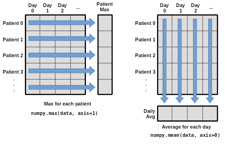
To support this functionality, most array functions allow us to specify the axis we want to work on. If we ask for the average across axis 0 (rows in our 2D example), we get:
OUTPUT
[  0.           0.45         1.11666667   1.75         2.43333333   3.15
   3.8          3.88333333   5.23333333   5.51666667   5.95         5.9
   8.35         7.73333333   8.36666667   9.5          9.58333333
  10.63333333  11.56666667  12.35        13.25        11.96666667
  11.03333333  10.16666667  10.           8.66666667   9.15         7.25
   7.33333333   6.58333333   6.06666667   5.95         5.11666667   3.6
   3.3          3.56666667   2.48333333   1.5          1.13333333
   0.56666667]
As a quick check, we can ask this array what its shape is:
OUTPUT
(40,)The expression (40,) tells us we have an N×1 vector, so
this is the average inflammation per day for all patients. If we average
across axis 1 (columns in our 2D example), we get:
OUTPUT
[ 5.45   5.425  6.1    5.9    5.55   6.225  5.975  6.65   6.625  6.525
  6.775  5.8    6.225  5.75   5.225  6.3    6.55   5.7    5.85   6.55
  5.775  5.825  6.175  6.1    5.8    6.425  6.05   6.025  6.175  6.55
  6.175  6.35   6.725  6.125  7.075  5.725  5.925  6.15   6.075  5.75
  5.975  5.725  6.3    5.9    6.75   5.925  7.225  6.15   5.95   6.275  5.7
  6.1    6.825  5.975  6.725  5.7    6.25   6.4    7.05   5.9  ]
which is the average inflammation per patient across all days.
Slicing Strings
A section of an array is called a slice. We can take slices of character strings as well:
PYTHON
element = 'oxygen'
print('first three characters:', element[0:3])
print('last three characters:', element[3:6])
OUTPUT
first three characters: oxy
last three characters: gen
What is the value of element[:4]? What about
element[4:]? Or element[:]?
OUTPUT
oxyg
en
oxygenSlicing Strings (continued)
What is element[-1]? What is
element[-2]?
OUTPUT
n
eSlicing Strings (continued)
Given those answers, explain what element[1:-1]
does.
Creates a substring from index 1 up to (not including) the final index, effectively removing the first and last letters from ‘oxygen’
Slicing Strings (continued)
How can we rewrite the slice for getting the last three characters of
element, so that it works even if we assign a different
string to element? Test your solution with the following
strings: carpentry, clone,
hi.
PYTHON
element = 'oxygen'
print('last three characters:', element[-3:])
element = 'carpentry'
print('last three characters:', element[-3:])
element = 'clone'
print('last three characters:', element[-3:])
element = 'hi'
print('last three characters:', element[-3:])
OUTPUT
last three characters: gen
last three characters: try
last three characters: one
last three characters: hiThin Slices
The expression element[3:3] produces an empty string, i.e., a string that
contains no characters. If data holds our array of patient
data, what does data[3:3, 4:4] produce? What about
data[3:3, :]?
OUTPUT
array([], shape=(0, 0), dtype=float64)
array([], shape=(0, 40), dtype=float64)Stacking Arrays
Arrays can be concatenated and stacked on top of one another, using
NumPy’s vstack and hstack functions for
vertical and horizontal stacking, respectively.
PYTHON
import numpy

A = numpy.array([[1, 2, 3], [4, 5, 6], [7, 8, 9]])
print('A = ')
print(A)

B = numpy.hstack([A, A])
print('B = ')
print(B)

C = numpy.vstack([A, A])
print('C = ')
print(C)
OUTPUT
A =
[[1 2 3]
 [4 5 6]
 [7 8 9]]
B =
[[1 2 3 1 2 3]
 [4 5 6 4 5 6]
 [7 8 9 7 8 9]]
C =
[[1 2 3]
 [4 5 6]
 [7 8 9]
 [1 2 3]
 [4 5 6]
 [7 8 9]]
Write some additional code that slices the first and last columns of
A, and stacks them into a 3x2 array. Make sure to
print the results to verify your solution.
A ‘gotcha’ with array indexing is that singleton dimensions are
dropped by default. That means A[:, 0] is a one dimensional
array, which won’t stack as desired. To preserve singleton dimensions,
the index itself can be a slice or array. For example,
A[:, :1] returns a two dimensional array with one singleton
dimension (i.e. a column vector).
OUTPUT
D =
[[1 3]
 [4 6]
[7 9]]Change In Inflammation
The patient data is longitudinal in the sense that each row represents a series of observations relating to one individual. This means that the change in inflammation over time is a meaningful concept. Let’s find out how to calculate changes in the data contained in an array with NumPy.
The numpy.diff() function takes an array and returns the
differences between two successive values. Let’s use it to examine the
changes each day across the first week of patient 3 from our
inflammation dataset.
OUTPUT
[0. 0. 2. 0. 4. 2. 2.]Calling numpy.diff(patient3_week1) would do the
following calculations
and return the 6 difference values in a new array.
OUTPUT
array([ 0., 2., -2., 4., -2., 0.])Note that the array of differences is shorter by one element (length 6).
When calling numpy.diff with a multi-dimensional array,
an axis argument may be passed to the function to specify
which axis to process. When applying numpy.diff to our 2D
inflammation array data, which axis would we specify?
Change In Inflammation (continued)
If the shape of an individual data file is (60, 40) (60
rows and 40 columns), what would the shape of the array be after you run
the diff() function and why?
The shape will be (60, 39) because there is one fewer
difference between columns than there are columns in the data.
Change In Inflammation (continued)
How would you find the largest change in inflammation for each patient? Does it matter if the change in inflammation is an increase or a decrease?
By using the numpy.amax() function after you apply the
numpy.diff() function, you will get the largest difference
between days.
PYTHON
array([  7.,  12.,  11.,  10.,  11.,  13.,  10.,   8.,  10.,  10.,   7.,
         7.,  13.,   7.,  10.,  10.,   8.,  10.,   9.,  10.,  13.,   7.,
        12.,   9.,  12.,  11.,  10.,  10.,   7.,  10.,  11.,  10.,   8.,
        11.,  12.,  10.,   9.,  10.,  13.,  10.,   7.,   7.,  10.,  13.,
        12.,   8.,   8.,  10.,  10.,   9.,   8.,  13.,  10.,   7.,  10.,
         8.,  12.,  10.,   7.,  12.])
If inflammation values decrease along an axis, then the
difference from one element to the next will be negative. If you are
interested in the magnitude of the change and not the
direction, the numpy.absolute() function will provide
that.
Notice the difference if you get the largest absolute difference between readings.
PYTHON
array([ 12.,  14.,  11.,  13.,  11.,  13.,  10.,  12.,  10.,  10.,  10.,
        12.,  13.,  10.,  11.,  10.,  12.,  13.,   9.,  10.,  13.,   9.,
        12.,   9.,  12.,  11.,  10.,  13.,   9.,  13.,  11.,  11.,   8.,
        11.,  12.,  13.,   9.,  10.,  13.,  11.,  11.,  13.,  11.,  13.,
        13.,  10.,   9.,  10.,  10.,   9.,   9.,  13.,  10.,   9.,  10.,
11., 13., 10., 10., 12.])- Import a library into a program using
import libraryname. - Use the
numpylibrary to work with arrays in Python. - The expression
array.shapegives the shape of an array. - Use
array[x, y]to select a single element from a 2D array. - Array indices start at 0, not 1.
- Use
low:highto specify aslicethat includes the indices fromlowtohigh-1. - Use
# some kind of explanationto add comments to programs. - Use
numpy.mean(array),numpy.amax(array), andnumpy.amin(array)to calculate simple statistics. - Use
numpy.mean(array, axis=0)ornumpy.mean(array, axis=1)to calculate statistics across the specified axis.
Content from Visualizing Tabular Data
Last updated on 2024-11-27 | Edit this page
Estimated time: 50 minutes
Overview
Questions
- How can I visualize tabular data in Python?
- How can I group several plots together?
Objectives
- Plot simple graphs from data.
- Plot multiple graphs in a single figure.
Visualizing data
The mathematician Richard Hamming once said, “The purpose of
computing is insight, not numbers,” and the best way to develop insight
is often to visualize data. Visualization deserves an entire lecture of
its own, but we can explore a few features of Python’s
matplotlib library here. While there is no official
plotting library, matplotlib is the de facto
standard. First, we will import the pyplot module from
matplotlib and use two of its functions to create and
display a heat map of our
data:
Episode Prerequisites

Each row in the heat map corresponds to a patient in the clinical trial dataset, and each column corresponds to a day in the dataset. Blue pixels in this heat map represent low values, while yellow pixels represent high values. As we can see, the general number of inflammation flare-ups for the patients rises and falls over a 40-day period.
So far so good as this is in line with our knowledge of the clinical trial and Dr. Maverick’s claims:
- the patients take their medication once their inflammation flare-ups begin
- it takes around 3 weeks for the medication to take effect and begin reducing flare-ups
- and flare-ups appear to drop to zero by the end of the clinical trial.
Now let’s take a look at the average inflammation over time:
PYTHON
ave_inflammation = numpy.mean(data, axis=0)
ave_plot = matplotlib.pyplot.plot(ave_inflammation)
matplotlib.pyplot.show()
Here, we have put the average inflammation per day across all
patients in the variable ave_inflammation, then asked
matplotlib.pyplot to create and display a line graph of
those values. The result is a reasonably linear rise and fall, in line
with Dr. Maverick’s claim that the medication takes 3 weeks to take
effect. But a good data scientist doesn’t just consider the average of a
dataset, so let’s have a look at two other statistics:


The maximum value rises and falls linearly, while the minimum seems to be a step function. Neither trend seems particularly likely, so either there’s a mistake in our calculations or something is wrong with our data. This insight would have been difficult to reach by examining the numbers themselves without visualization tools.
Grouping plots
You can group similar plots in a single figure using subplots. This
script below uses a number of new commands. The function
matplotlib.pyplot.figure() creates a space into which we
will place all of our plots. The parameter figsize tells
Python how big to make this space. Each subplot is placed into the
figure using its add_subplot method. The add_subplot
method takes 3 parameters. The first denotes how many total rows of
subplots there are, the second parameter refers to the total number of
subplot columns, and the final parameter denotes which subplot your
variable is referencing (left-to-right, top-to-bottom). Each subplot is
stored in a different variable (axes1, axes2,
axes3). Once a subplot is created, the axes can be titled
using the set_xlabel() command (or
set_ylabel()). Here are our three plots side by side:
PYTHON
import numpy
import matplotlib.pyplot

data = numpy.loadtxt(fname='inflammation-01.csv', delimiter=',')

fig = matplotlib.pyplot.figure(figsize=(10.0, 3.0))

axes1 = fig.add_subplot(1, 3, 1)
axes2 = fig.add_subplot(1, 3, 2)
axes3 = fig.add_subplot(1, 3, 3)

axes1.set_ylabel('average')
axes1.plot(numpy.mean(data, axis=0))

axes2.set_ylabel('max')
axes2.plot(numpy.amax(data, axis=0))

axes3.set_ylabel('min')
axes3.plot(numpy.amin(data, axis=0))

fig.tight_layout()

matplotlib.pyplot.savefig('inflammation.png')
matplotlib.pyplot.show()
The call to
loadtxt reads our data, and the rest of the program tells
the plotting library how large we want the figure to be, that we’re
creating three subplots, what to draw for each one, and that we want a
tight layout. (If we leave out that call to
fig.tight_layout(), the graphs will actually be squeezed
together more closely.)
The call to savefig stores the plot as a graphics file.
This can be a convenient way to store your plots for use in other
documents, web pages etc. The graphics format is automatically
determined by Matplotlib from the file name ending we specify; here PNG
from ‘inflammation.png’. Matplotlib supports many different graphics
formats, including SVG, PDF, and JPEG.
Importing libraries with shortcuts
In this lesson we use the import matplotlib.pyplot syntax to import the
pyplot module of matplotlib. However,
shortcuts such as import matplotlib.pyplot as plt are
frequently used. Importing pyplot this way means that after
the initial import, rather than writing
matplotlib.pyplot.plot(...), you can now write
plt.plot(...). Another common convention is to use the
shortcut import numpy as np when importing the NumPy
library. We then can write np.loadtxt(...) instead of
numpy.loadtxt(...), for example.
Some people prefer these shortcuts as it is quicker to type and
results in shorter lines of code - especially for libraries with long
names! You will frequently see Python code online using a
pyplot function with plt, or a NumPy function
with np, and it’s because they’ve used this shortcut. It
makes no difference which approach you choose to take, but you must be
consistent as if you use import matplotlib.pyplot as plt
then matplotlib.pyplot.plot(...) will not work, and you
must use plt.plot(...) instead. Because of this, when
working with other people it is important you agree on how libraries are
imported.
Plot Scaling
Why do all of our plots stop just short of the upper end of our graph?
Because matplotlib normally sets x and y axes limits to the min and max of our data (depending on data range)
Drawing Straight Lines
In the center and right subplots above, we expect all lines to look like step functions because non-integer value are not realistic for the minimum and maximum values. However, you can see that the lines are not always vertical or horizontal, and in particular the step function in the subplot on the right looks slanted. Why is this?
Because matplotlib interpolates (draws a straight line) between the
points. One way to do avoid this is to use the Matplotlib
drawstyle option:
PYTHON
import numpy
import matplotlib.pyplot

data = numpy.loadtxt(fname='inflammation-01.csv', delimiter=',')

fig = matplotlib.pyplot.figure(figsize=(10.0, 3.0))

axes1 = fig.add_subplot(1, 3, 1)
axes2 = fig.add_subplot(1, 3, 2)
axes3 = fig.add_subplot(1, 3, 3)

axes1.set_ylabel('average')
axes1.plot(numpy.mean(data, axis=0), drawstyle='steps-mid')

axes2.set_ylabel('max')
axes2.plot(numpy.amax(data, axis=0), drawstyle='steps-mid')

axes3.set_ylabel('min')
axes3.plot(numpy.amin(data, axis=0), drawstyle='steps-mid')

fig.tight_layout()

matplotlib.pyplot.show()
Make Your Own Plot
Create a plot showing the standard deviation (numpy.std)
of the inflammation data for each day across all patients.
Moving Plots Around
Modify the program to display the three plots on top of one another instead of side by side.
PYTHON
import numpy
import matplotlib.pyplot

data = numpy.loadtxt(fname='inflammation-01.csv', delimiter=',')

# change figsize (swap width and height)
fig = matplotlib.pyplot.figure(figsize=(3.0, 10.0))

# change add_subplot (swap first two parameters)
axes1 = fig.add_subplot(3, 1, 1)
axes2 = fig.add_subplot(3, 1, 2)
axes3 = fig.add_subplot(3, 1, 3)

axes1.set_ylabel('average')
axes1.plot(numpy.mean(data, axis=0))

axes2.set_ylabel('max')
axes2.plot(numpy.amax(data, axis=0))

axes3.set_ylabel('min')
axes3.plot(numpy.amin(data, axis=0))

fig.tight_layout()

matplotlib.pyplot.show()- Use the
pyplotmodule from thematplotliblibrary for creating simple visualizations.
Content from Creating Functions
Last updated on 2024-11-27 | Edit this page
Estimated time: 30 minutes
Overview
Questions
- How can I define new functions?
- What’s the difference between defining and calling a function?
- What happens when I call a function?
Objectives
- Define a function that takes parameters.
- Return a value from a function.
- Test and debug a function.
- Set default values for function parameters.
- Explain why we should divide programs into small, single-purpose functions.
At this point, we’ve seen that code can have Python make decisions about what it sees in our data. What if we want to convert some of our data, like taking a temperature in Fahrenheit and converting it to Celsius. We could write something like this for converting a single number
and for a second number we could just copy the line and rename the variables
PYTHON
fahrenheit_val = 99
celsius_val = ((fahrenheit_val - 32) * (5/9))
fahrenheit_val2 = 43
celsius_val2 = ((fahrenheit_val2 - 32) * (5/9))But we would be in trouble as soon as we had to do this more than a
couple times. Cutting and pasting it is going to make our code get very
long and very repetitive, very quickly. We’d like a way to package our
code so that it is easier to reuse, a shorthand way of re-executing
longer pieces of code. In Python we can use ‘functions’. Let’s start by
defining a function fahr_to_celsius that converts
temperatures from Fahrenheit to Celsius:
PYTHON
def explicit_fahr_to_celsius(temp):
    # Assign the converted value to a variable
    converted = ((temp - 32) * (5/9))
    # Return the value of the new variable
    return converted

def fahr_to_celsius(temp):
    # Return converted value more efficiently using the return
    # function without creating a new variable. This code does
    # the same thing as the previous function but it is more explicit
    # in explaining how the return command works.
    return ((temp - 32) * (5/9))
The function definition opens with the keyword def
followed by the name of the function (fahr_to_celsius) and
a parenthesized list of parameter names (temp). The body of the function — the statements
that are executed when it runs — is indented below the definition line.
The body concludes with a return keyword followed by the
return value.
When we call the function, the values we pass to it are assigned to those variables so that we can use them inside the function. Inside the function, we use a return statement to send a result back to whoever asked for it.
Let’s try running our function.
This command should call our function, using 32 as the
input and return the function value.
In fact, calling our own function is no different from calling any other function:
PYTHON
print(f'freezing point of water: {fahr_to_celsius(32)}ºC')
print(f'boiling point of water: {fahr_to_celsius(212)}ºC')
OUTPUT
freezing point of water: 0.0ºC
boiling point of water: 100.0ºC
We’ve successfully called the function that we defined, and we have access to the value that we returned.
Composing Functions
Now that we’ve seen how to turn Fahrenheit into Celsius, we can also write the function to turn Celsius into Kelvin:
PYTHON
def celsius_to_kelvin(temp_c):
return temp_c + 273.15
print(f'freezing point of water: {celsius_to_kelvin(0.)}ºK')OUTPUT
freezing point of water: 273.15ºKWhat about converting Fahrenheit to Kelvin? We could write out the formula, but we don’t need to. Instead, we can compose the two functions we have already created:
PYTHON
def fahr_to_kelvin(temp_f):
temp_c = fahr_to_celsius(temp_f)
temp_k = celsius_to_kelvin(temp_c)
return temp_k
print(f'boiling point of water: {fahr_to_kelvin(212.)ºK}')OUTPUT
boiling point of water: 373.15ºKThis is our first taste of how larger programs are built: we define basic operations, then combine them in ever-larger chunks to get the effect we want. Real-life functions will usually be larger than the ones shown here — typically half a dozen to a few dozen lines — but they shouldn’t ever be much longer than that, or the next person who reads it won’t be able to understand what’s going on.
Variable Scope
In composing our temperature conversion functions, we created
variables inside of those functions, temp,
temp_c, temp_f, and temp_k. We
refer to these variables as local variables because they no
longer exist once the function is done executing. If we try to access
their values outside of the function, we will encounter an error:
ERROR
---------------------------------------------------------------------------
NameError Traceback (most recent call last)
<ipython-input-1-eed2471d229b> in <module>
----> 1 print('Again, temperature in Kelvin was:', temp_k)
NameError: name 'temp_k' is not definedIf you want to reuse the temperature in Kelvin after you have
calculated it with fahr_to_kelvin, you can store the result
of the function call in a variable:
PYTHON
temp_kelvin = fahr_to_kelvin(212.0)
print(f'temperature in degrees Kelvin was: {temp_kelvin}')OUTPUT
temperature in degrees Kelvin was: 373.15The variable temp_kelvin, being defined outside any
function, is said to be global.
Inside a function, one can read the value of such global variables:
PYTHON
def print_temperatures():
print(f'temperature in degrees Fahrenheit was: {temp_fahr}')
print(f'temperature in degrees Kelvin was: {temp_kelvin}')
temp_fahr = 212.0
temp_kelvin = fahr_to_kelvin(temp_fahr)
print_temperatures()OUTPUT
temperature in degrees Fahrenheit was: 212.0
temperature in degrees Kelvin was: 373.15Tidying up
Now that we know how to wrap bits of code up in functions, we can
make our inflammation analysis easier to read and easier to reuse.
First, let’s make a visualize function that generates our
plots:
PYTHON
def visualize(filename):
data = numpy.loadtxt(fname=filename, delimiter=',')
fig = matplotlib.pyplot.figure(figsize=(10.0, 3.0))
axes1 = fig.add_subplot(1, 3, 1)
axes2 = fig.add_subplot(1, 3, 2)
axes3 = fig.add_subplot(1, 3, 3)
axes1.set_ylabel('average')
axes1.plot(numpy.mean(data, axis=0))
axes2.set_ylabel('max')
axes2.plot(numpy.amax(data, axis=0))
axes3.set_ylabel('min')
axes3.plot(numpy.amin(data, axis=0))
fig.tight_layout()
matplotlib.pyplot.show()and another function called detect_problems that checks
for those systematics we noticed:
PYTHON
def detect_problems(filename):
data = numpy.loadtxt(fname=filename, delimiter=',')
if numpy.amax(data, axis=0)[0] == 0 and numpy.amax(data, axis=0)[20] == 20:
print('Suspicious looking maxima!')
elif numpy.sum(numpy.amin(data, axis=0)) == 0:
print('Minima add up to zero!')
else:
print('Seems OK!')Wait! Didn’t we forget to specify what both of these functions should
return? Well, we didn’t. In Python, functions are not required to
include a return statement and can be used for the sole
purpose of grouping together pieces of code that conceptually do one
thing. In such cases, function names usually describe what they do,
e.g. visualize, detect_problems.
Notice that rather than jumbling this code together in one giant
for loop, we can now read and reuse both ideas separately.
We can reproduce the previous analysis with a much simpler
for loop:
PYTHON
filenames = sorted(glob.glob('inflammation*.csv'))
for filename in filenames[:3]:
print(filename)
visualize(filename)
detect_problems(filename)By giving our functions human-readable names, we can more easily read
and understand what is happening in the for loop. Even
better, if at some later date we want to use either of those pieces of
code again, we can do so in a single line.
Testing and Documenting
Once we start putting things in functions so that we can re-use them, we need to start testing that those functions are working correctly. To see how to do this, let’s write a function to offset a dataset so that it’s mean value shifts to a user-defined value:
PYTHON
def offset_mean(data, target_mean_value):
return (data - numpy.mean(data)) + target_mean_valueWe could test this on our actual data, but since we don’t know what the values ought to be, it will be hard to tell if the result was correct. Instead, let’s use NumPy to create a matrix of 0’s and then offset its values to have a mean value of 3:
OUTPUT
[[ 3. 3.]
[ 3. 3.]]That looks right, so let’s try offset_mean on our real
data:
OUTPUT
[[-6.14875 -6.14875 -5.14875 ... -3.14875 -6.14875 -6.14875]
[-6.14875 -5.14875 -4.14875 ... -5.14875 -6.14875 -5.14875]
[-6.14875 -5.14875 -5.14875 ... -4.14875 -5.14875 -5.14875]
...
[-6.14875 -5.14875 -5.14875 ... -5.14875 -5.14875 -5.14875]
[-6.14875 -6.14875 -6.14875 ... -6.14875 -4.14875 -6.14875]
[-6.14875 -6.14875 -5.14875 ... -5.14875 -5.14875 -6.14875]]It’s hard to tell from the default output whether the result is correct, but there are a few tests that we can run to reassure us:
PYTHON
print('original min, mean, and max are:', numpy.amin(data), numpy.mean(data), numpy.amax(data))
offset_data = offset_mean(data, 0)
print('min, mean, and max of offset data are:',
numpy.amin(offset_data),
numpy.mean(offset_data),
numpy.amax(offset_data))OUTPUT
original min, mean, and max are: 0.0 6.14875 20.0
min, mean, and max of offset data are: -6.14875 2.842170943040401e-16 13.85125That seems almost right: the original mean was about 6.1, so the lower bound from zero is now about -6.1. The mean of the offset data isn’t quite zero, but it’s pretty close. We can even go further and check that the standard deviation hasn’t changed:
OUTPUT
std dev before and after: 4.613833197118566 4.613833197118566Those values look the same, but we probably wouldn’t notice if they were different in the sixth decimal place. Let’s do this instead:
PYTHON
print('difference in standard deviations before and after:',
numpy.std(data) - numpy.std(offset_data))OUTPUT
difference in standard deviations before and after: 0.0Everything looks good, and we should probably get back to doing our analysis. We have one more task first, though: we should write some documentation for our function to remind ourselves later what it’s for and how to use it.
The usual way to put documentation in software is to add comments like this:
PYTHON
# offset_mean(data, target_mean_value):
# return a new array containing the original data with its mean offset to match the desired value.
def offset_mean(data, target_mean_value):
return (data - numpy.mean(data)) + target_mean_valueThere’s a better way, though. If the first thing in a function is a string that isn’t assigned to a variable, that string is attached to the function as its documentation:
PYTHON
def offset_mean(data, target_mean_value):
"""Return a new array containing the original data
with its mean offset to match the desired value."""
return (data - numpy.mean(data)) + target_mean_valueThis is better because we can now ask Python’s built-in help system to show us the documentation for the function:
OUTPUT
Help on function offset_mean in module __main__:
offset_mean(data, target_mean_value)
Return a new array containing the original data with its mean offset to match the desired value.A string like this is called a docstring. We don’t need to use triple quotes when we write one, but if we do, we can break the string across multiple lines:
PYTHON
def offset_mean(data, target_mean_value):
"""Return a new array containing the original data
with its mean offset to match the desired value.
Examples
--------
>>> offset_mean([1, 2, 3], 0)
array([-1., 0., 1.])
"""
return (data - numpy.mean(data)) + target_mean_value
help(offset_mean)OUTPUT
Help on function offset_mean in module __main__:
offset_mean(data, target_mean_value)
Return a new array containing the original data
with its mean offset to match the desired value.
Examples
--------
>>> offset_mean([1, 2, 3], 0)
array([-1., 0., 1.])Defining Defaults
We have passed parameters to functions in two ways: directly, as in
type(data), and by name, as in
numpy.loadtxt(fname='something.csv', delimiter=','). In
fact, we can pass the filename to loadtxt without the
fname=:
OUTPUT
array([[ 0., 0., 1., ..., 3., 0., 0.],
[ 0., 1., 2., ..., 1., 0., 1.],
[ 0., 1., 1., ..., 2., 1., 1.],
...,
[ 0., 1., 1., ..., 1., 1., 1.],
[ 0., 0., 0., ..., 0., 2., 0.],
[ 0., 0., 1., ..., 1., 1., 0.]])but we still need to say delimiter=:
ERROR
Traceback (most recent call last):
File "<stdin>", line 1, in <module>
File "/Users/username/anaconda3/lib/python3.6/site-packages/numpy/lib/npyio.py", line 1041, in loa
dtxt
dtype = np.dtype(dtype)
File "/Users/username/anaconda3/lib/python3.6/site-packages/numpy/core/_internal.py", line 199, in
_commastring
newitem = (dtype, eval(repeats))
File "<string>", line 1
,
^
SyntaxError: unexpected EOF while parsingTo understand what’s going on, and make our own functions easier to
use, let’s re-define our offset_mean function like
this:
PYTHON
def offset_mean(data, target_mean_value=0.0):
"""Return a new array containing the original data
with its mean offset to match the desired value, (0 by default).
Examples
--------
>>> offset_mean([1, 2, 3])
array([-1., 0., 1.])
"""
return (data - numpy.mean(data)) + target_mean_valueThe key change is that the second parameter is now written
target_mean_value=0.0 instead of just
target_mean_value. If we call the function with two
arguments, it works as it did before:
OUTPUT
[[ 3. 3.]
[ 3. 3.]]But we can also now call it with just one parameter, in which case
target_mean_value is automatically assigned the default value of 0.0:
PYTHON
more_data = 5 + numpy.zeros((2, 2))
print('data before mean offset:')
print(more_data)
print('offset data:')
print(offset_mean(more_data))OUTPUT
data before mean offset:
[[ 5. 5.]
[ 5. 5.]]
offset data:
[[ 0. 0.]
[ 0. 0.]]This is handy: if we usually want a function to work one way, but occasionally need it to do something else, we can allow people to pass a parameter when they need to but provide a default to make the normal case easier. The example below shows how Python matches values to parameters:
PYTHON
def display(a=1, b=2, c=3):
print('a:', a, 'b:', b, 'c:', c)
print('no parameters:')
display()
print('one parameter:')
display(55)
print('two parameters:')
display(55, 66)OUTPUT
no parameters:
a: 1 b: 2 c: 3
one parameter:
a: 55 b: 2 c: 3
two parameters:
a: 55 b: 66 c: 3As this example shows, parameters are matched up from left to right, and any that haven’t been given a value explicitly get their default value. We can override this behavior by naming the value as we pass it in:
OUTPUT
only setting the value of c
a: 1 b: 2 c: 77With that in hand, let’s look at the help for
numpy.loadtxt:
OUTPUT
Help on function loadtxt in module numpy.lib.npyio:
loadtxt(fname, dtype=<class 'float'>, comments='#', delimiter=None, converters=None, skiprows=0, use
cols=None, unpack=False, ndmin=0, encoding='bytes')
Load data from a text file.
Each row in the text file must have the same number of values.
Parameters
----------
...There’s a lot of information here, but the most important part is the first couple of lines:
OUTPUT
loadtxt(fname, dtype=<class 'float'>, comments='#', delimiter=None, converters=None, skiprows=0, use
cols=None, unpack=False, ndmin=0, encoding='bytes')This tells us that loadtxt has one parameter called
fname that doesn’t have a default value, and eight others
that do. If we call the function like this:
then the filename is assigned to fname (which is what we
want), but the delimiter string ',' is assigned to
dtype rather than delimiter, because
dtype is the second parameter in the list. However
',' isn’t a known dtype so our code produced
an error message when we tried to run it. When we call
loadtxt we don’t have to provide fname= for
the filename because it’s the first item in the list, but if we want the
',' to be assigned to the variable delimiter,
we do have to provide delimiter= for the second
parameter since delimiter is not the second parameter in
the list.
Readable functions
Consider these two functions:
PYTHON
def s(p):
a = 0
for v in p:
a += v
m = a / len(p)
d = 0
for v in p:
d += (v - m) * (v - m)
return numpy.sqrt(d / (len(p) - 1))
def std_dev(sample):
sample_sum = 0
for value in sample:
sample_sum += value
sample_mean = sample_sum / len(sample)
sum_squared_devs = 0
for value in sample:
sum_squared_devs += (value - sample_mean) * (value - sample_mean)
return numpy.sqrt(sum_squared_devs / (len(sample) - 1))The functions s and std_dev are
computationally equivalent (they both calculate the sample standard
deviation), but to a human reader, they look very different. You
probably found std_dev much easier to read and understand
than s.
As this example illustrates, both documentation and a programmer’s coding style combine to determine how easy it is for others to read and understand the programmer’s code. Choosing meaningful variable names and using blank spaces to break the code into logical “chunks” are helpful techniques for producing readable code. This is useful not only for sharing code with others, but also for the original programmer. If you need to revisit code that you wrote months ago and haven’t thought about since then, you will appreciate the value of readable code!
Combining Strings
“Adding” two strings produces their concatenation:
'a' + 'b' is 'ab'. Write a function called
fence that takes two parameters called
original and wrapper and returns a new string
that has the wrapper character at the beginning and end of the original.
A call to your function should look like this:
OUTPUT
*name*Return versus print
Note that return and print are not
interchangeable. print is a Python function that
prints data to the screen. It enables us, users, see
the data. return statement, on the other hand, makes data
visible to the program. Let’s have a look at the following function:
Question: What will we see if we execute the following commands?
Python will first execute the function add with
a = 7 and b = 3, and, therefore, print
10. However, because function add does not
have a line that starts with return (no return
“statement”), it will, by default, return nothing which, in Python
world, is called None. Therefore, A will be
assigned to None and the last line (print(A))
will print None. As a result, we will see:
OUTPUT
10
NoneSelecting Characters From Strings
If the variable s refers to a string, then
s[0] is the string’s first character and s[-1]
is its last. Write a function called outer that returns a
string made up of just the first and last characters of its input. A
call to your function should look like this:
OUTPUT
hmRescaling an Array
Write a function rescale that takes an array as input
and returns a corresponding array of values scaled to lie in the range
0.0 to 1.0. (Hint: If L and H are the lowest
and highest values in the original array, then the replacement for a
value v should be (v-L) / (H-L).)
Testing and Documenting Your Function
Run the commands help(numpy.arange) and
help(numpy.linspace) to see how to use these functions to
generate regularly-spaced values, then use those values to test your
rescale function. Once you’ve successfully tested your
function, add a docstring that explains what it does.
PYTHON
"""Takes an array as input, and returns a corresponding array scaled so
that 0 corresponds to the minimum and 1 to the maximum value of the input array.
Examples:
>>> rescale(numpy.arange(10.0))
array([ 0. , 0.11111111, 0.22222222, 0.33333333, 0.44444444,
0.55555556, 0.66666667, 0.77777778, 0.88888889, 1. ])
>>> rescale(numpy.linspace(0, 100, 5))
array([ 0. , 0.25, 0.5 , 0.75, 1. ])
"""Defining Defaults
Rewrite the rescale function so that it scales data to
lie between 0.0 and 1.0 by default, but will
allow the caller to specify lower and upper bounds if they want. Compare
your implementation to your neighbor’s: do the two functions always
behave the same way?
PYTHON
def rescale(input_array, low_val=0.0, high_val=1.0):
"""rescales input array values to lie between low_val and high_val"""
L = numpy.amin(input_array)
H = numpy.amax(input_array)
intermed_array = (input_array - L) / (H - L)
output_array = intermed_array * (high_val - low_val) + low_val
return output_arrayOUTPUT
259.81666666666666
278.15
273.15
0k is 0 because the k inside the function
f2k doesn’t know about the k defined outside
the function. When the f2k function is called, it creates a
local variable
k. The function does not return any values and does not
alter k outside of its local copy. Therefore the original
value of k remains unchanged. Beware that a local
k is created because f2k internal statements
affect a new value to it. If k was only
read, it would simply retrieve the global k
value.
Mixing Default and Non-Default Parameters
Given the following code:
PYTHON
def numbers(one, two=2, three, four=4):
n = str(one) + str(two) + str(three) + str(four)
return n
print(numbers(1, three=3))what do you expect will be printed? What is actually printed? What rule do you think Python is following?
1234one2three41239SyntaxError
Given that, what does the following piece of code display when run?
a: b: 3 c: 6a: -1 b: 3 c: 6a: -1 b: 2 c: 6a: b: -1 c: 2
Attempting to define the numbers function results in
4. SyntaxError. The defined parameters two and
four are given default values. Because one and
three are not given default values, they are required to be
included as arguments when the function is called and must be placed
before any parameters that have default values in the function
definition.
The given call to func displays
a: -1 b: 2 c: 6. -1 is assigned to the first parameter
a, 2 is assigned to the next parameter b, and
c is not passed a value, so it uses its default value
6.
Readable Code
Revise a function you wrote for one of the previous exercises to try to make the code more readable. Then, collaborate with one of your neighbors to critique each other’s functions and discuss how your function implementations could be further improved to make them more readable.
- Define a function using
def function_name(parameter). - The body of a function must be indented.
- Call a function using
function_name(value). - Numbers are stored as integers or floating-point numbers.
- Variables defined within a function can only be seen and used within the body of the function.
- Variables created outside of any function are called global variables.
- Within a function, we can access global variables.
- Variables created within a function override global variables if their names match.
- Use
help(thing)to view help for something. - Put docstrings in functions to provide help for that function.
- Specify default values for parameters when defining a function using
name=valuein the parameter list. - Parameters can be passed by matching based on name, by position, or by omitting them (in which case the default value is used).
- Put code whose parameters change frequently in a function, then call it with different parameter values to customize its behavior.
Content from Analyzing Data from Multiple Files
Last updated on 2024-11-27 | Edit this page
Estimated time: 20 minutes
Overview
Questions
- How can I do the same operations on many different files?
Objectives
- Use a library function to get a list of filenames that match a wildcard pattern.
- Write a
forloop to process multiple files.
As a final piece to processing our inflammation data, we need a way
to get a list of all the files in our data directory whose
names start with inflammation- and end with
.csv. The following library will help us to achieve
this:
The glob library contains a function, also called
glob, that finds files and directories whose names match a
pattern. We provide those patterns as strings: the character
* matches zero or more characters, while ?
matches any one character. We can use this to get the names of all the
CSV files in the current directory:
OUTPUT
['inflammation-05.csv', 'inflammation-11.csv', 'inflammation-12.csv', 'inflammation-08.csv',
'inflammation-03.csv', 'inflammation-06.csv', 'inflammation-09.csv', 'inflammation-07.csv',
'inflammation-10.csv', 'inflammation-02.csv', 'inflammation-04.csv', 'inflammation-01.csv']As these examples show, glob.glob’s result is a list of
file and directory paths in arbitrary order. This means we can loop over
it to do something with each filename in turn. In our case, the
“something” we want to do is generate a set of plots for each file in
our inflammation dataset.
If we want to start by analyzing just the first three files in
alphabetical order, we can use the sorted built-in function
to generate a new sorted list from the glob.glob
output:
PYTHON
import glob
import numpy
import matplotlib.pyplot
filenames = sorted(glob.glob('inflammation*.csv'))
filenames = filenames[0:3]
for filename in filenames:
print(filename)
data = numpy.loadtxt(fname=filename, delimiter=',')
fig = matplotlib.pyplot.figure(figsize=(10.0, 3.0))
axes1 = fig.add_subplot(1, 3, 1)
axes2 = fig.add_subplot(1, 3, 2)
axes3 = fig.add_subplot(1, 3, 3)
axes1.set_ylabel('average')
axes1.plot(numpy.mean(data, axis=0))
axes2.set_ylabel('max')
axes2.plot(numpy.amax(data, axis=0))
axes3.set_ylabel('min')
axes3.plot(numpy.amin(data, axis=0))
fig.tight_layout()
matplotlib.pyplot.show()OUTPUT
inflammation-01.csv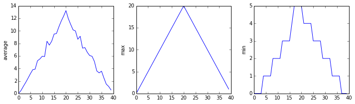
OUTPUT
inflammation-02.csv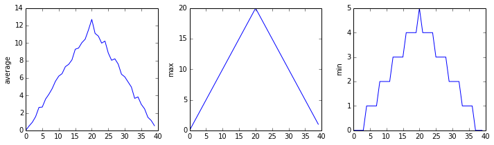
OUTPUT
inflammation-03.csv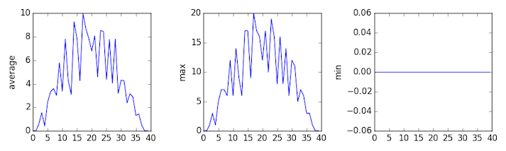
The plots generated for the second clinical trial file look very similar to the plots for the first file: their average plots show similar “noisy” rises and falls; their maxima plots show exactly the same linear rise and fall; and their minima plots show similar staircase structures.
The third dataset shows much noisier average and maxima plots that are far less suspicious than the first two datasets, however the minima plot shows that the third dataset minima is consistently zero across every day of the trial. If we produce a heat map for the third data file we see the following:

We can see that there are zero values sporadically distributed across all patients and days of the clinical trial, suggesting that there were potential issues with data collection throughout the trial. In addition, we can see that the last patient in the study didn’t have any inflammation flare-ups at all throughout the trial, suggesting that they may not even suffer from arthritis!
Plotting Differences
Plot the difference between the average inflammations reported in the
first and second datasets (stored in inflammation-01.csv
and inflammation-02.csv, correspondingly), i.e., the
difference between the leftmost plots of the first two figures.
PYTHON
import glob
import numpy
import matplotlib.pyplot
filenames = sorted(glob.glob('inflammation*.csv'))
data0 = numpy.loadtxt(fname=filenames[0], delimiter=',')
data1 = numpy.loadtxt(fname=filenames[1], delimiter=',')
fig = matplotlib.pyplot.figure(figsize=(10.0, 3.0))
matplotlib.pyplot.ylabel('Difference in average')
matplotlib.pyplot.plot(numpy.mean(data0, axis=0) - numpy.mean(data1, axis=0))
fig.tight_layout()
matplotlib.pyplot.show()Generate Composite Statistics
Use each of the files once to generate a dataset containing values averaged over all patients by completing the code inside the loop given below:
PYTHON
filenames = glob.glob('inflammation*.csv')
composite_data = numpy.zeros((60, 40))
for filename in filenames:
# sum each new file's data into composite_data as it's read
#
# and then divide the composite_data by number of samples
composite_data = composite_data / len(filenames)Then use pyplot to generate average, max, and min for all patients.
PYTHON
import glob
import numpy
import matplotlib.pyplot
filenames = glob.glob('inflammation*.csv')
composite_data = numpy.zeros((60, 40))
for filename in filenames:
data = numpy.loadtxt(fname = filename, delimiter=',')
composite_data = composite_data + data
composite_data = composite_data / len(filenames)
fig = matplotlib.pyplot.figure(figsize=(10.0, 3.0))
axes1 = fig.add_subplot(1, 3, 1)
axes2 = fig.add_subplot(1, 3, 2)
axes3 = fig.add_subplot(1, 3, 3)
axes1.set_ylabel('average')
axes1.plot(numpy.mean(composite_data, axis=0))
axes2.set_ylabel('max')
axes2.plot(numpy.amax(composite_data, axis=0))
axes3.set_ylabel('min')
axes3.plot(numpy.amin(composite_data, axis=0))
fig.tight_layout()
matplotlib.pyplot.show()After spending some time investigating the heat map and statistical plots, as well as doing the above exercises to plot differences between datasets and to generate composite patient statistics, we gain some insight into the twelve clinical trial datasets.
The datasets appear to fall into two categories:
- seemingly “ideal” datasets that agree excellently with
Dr. Maverick’s claims, but display suspicious maxima and minima (such as
inflammation-01.csvandinflammation-02.csv) - “noisy” datasets that somewhat agree with Dr. Maverick’s claims, but show concerning data collection issues such as sporadic missing values and even an unsuitable candidate making it into the clinical trial.
In fact, it appears that all three of the “noisy” datasets
(inflammation-03.csv, inflammation-08.csv, and
inflammation-11.csv) are identical down to the last value.
Armed with this information, we confront Dr. Maverick about the
suspicious data and duplicated files.
Dr. Maverick has admitted to fabricating the clinical data for their drug trial. They did this after discovering that the initial trial had several issues, including unreliable data recording and poor participant selection. In order to prove the efficacy of their drug, they created fake data. When asked for additional data, they attempted to generate more fake datasets, and also included the original poor-quality dataset several times in order to make the trials seem more realistic.
Congratulations! We’ve investigated the inflammation data and proven that the datasets have been synthetically generated.
But it would be a shame to throw away the synthetic datasets that have taught us so much already, so we’ll forgive the imaginary Dr. Maverick and continue to use the data to learn how to program.
- Use
glob.glob(pattern)to create a list of files whose names match a pattern. - Use
*in a pattern to match zero or more characters, and?to match any single character.
Content from Errors and Exceptions
Last updated on 2023-04-21 | Edit this page
Estimated time: 30 minutes
Overview
Questions
- How does Python report errors?
- How can I handle errors in Python programs?
Objectives
- To be able to read a traceback, and determine where the error took place and what type it is.
- To be able to describe the types of situations in which syntax errors, indentation errors, name errors, index errors, and missing file errors occur.
Every programmer encounters errors, both those who are just beginning, and those who have been programming for years. Encountering errors and exceptions can be very frustrating at times, and can make coding feel like a hopeless endeavour. However, understanding what the different types of errors are and when you are likely to encounter them can help a lot. Once you know why you get certain types of errors, they become much easier to fix.
Errors in Python have a very specific form, called a traceback. Let’s examine one:
PYTHON
# This code has an intentional error. You can type it directly or
# use it for reference to understand the error message below.
def favorite_ice_cream():
ice_creams = [
'chocolate',
'vanilla',
'strawberry'
]
print(ice_creams[3])
favorite_ice_cream()ERROR
---------------------------------------------------------------------------
IndexError Traceback (most recent call last)
<ipython-input-1-70bd89baa4df> in <module>()
9 print(ice_creams[3])
10
----> 11 favorite_ice_cream()
<ipython-input-1-70bd89baa4df> in favorite_ice_cream()
7 'strawberry'
8 ]
----> 9 print(ice_creams[3])
10
11 favorite_ice_cream()
IndexError: list index out of rangeThis particular traceback has two levels. You can determine the number of levels by looking for the number of arrows on the left hand side. In this case:
The first shows code from the cell above, with an arrow pointing to Line 11 (which is
favorite_ice_cream()).The second shows some code in the function
favorite_ice_cream, with an arrow pointing to Line 9 (which isprint(ice_creams[3])).
The last level is the actual place where the error occurred. The
other level(s) show what function the program executed to get to the
next level down. So, in this case, the program first performed a function call to the function
favorite_ice_cream. Inside this function, the program
encountered an error on Line 6, when it tried to run the code
print(ice_creams[3]).
Long Tracebacks
Sometimes, you might see a traceback that is very long -- sometimes they might even be 20 levels deep! This can make it seem like something horrible happened, but the length of the error message does not reflect severity, rather, it indicates that your program called many functions before it encountered the error. Most of the time, the actual place where the error occurred is at the bottom-most level, so you can skip down the traceback to the bottom.
So what error did the program actually encounter? In the last line of
the traceback, Python helpfully tells us the category or type of error
(in this case, it is an IndexError) and a more detailed
error message (in this case, it says “list index out of range”).
If you encounter an error and don’t know what it means, it is still important to read the traceback closely. That way, if you fix the error, but encounter a new one, you can tell that the error changed. Additionally, sometimes knowing where the error occurred is enough to fix it, even if you don’t entirely understand the message.
If you do encounter an error you don’t recognize, try looking at the official documentation on errors. However, note that you may not always be able to find the error there, as it is possible to create custom errors. In that case, hopefully the custom error message is informative enough to help you figure out what went wrong.
Reading Error Messages
Read the Python code and the resulting traceback below, and answer the following questions:
- How many levels does the traceback have?
- What is the function name where the error occurred?
- On which line number in this function did the error occur?
- What is the type of error?
- What is the error message?
PYTHON
# This code has an intentional error. Do not type it directly;
# use it for reference to understand the error message below.
def print_message(day):
messages = [
'Hello, world!',
'Today is Tuesday!',
'It is the middle of the week.',
'Today is Donnerstag in German!',
'Last day of the week!',
'Hooray for the weekend!',
'Aw, the weekend is almost over.'
]
print(messages[day])
def print_sunday_message():
print_message(7)
print_sunday_message()ERROR
---------------------------------------------------------------------------
IndexError Traceback (most recent call last)
<ipython-input-7-3ad455d81842> in <module>
16 print_message(7)
17
---> 18 print_sunday_message()
19
<ipython-input-7-3ad455d81842> in print_sunday_message()
14
15 def print_sunday_message():
---> 16 print_message(7)
17
18 print_sunday_message()
<ipython-input-7-3ad455d81842> in print_message(day)
11 'Aw, the weekend is almost over.'
12 ]
---> 13 print(messages[day])
14
15 def print_sunday_message():
IndexError: list index out of range- 3 levels
print_message- 13
IndexError-
list index out of rangeYou can then infer that7is not the right index to use withmessages.
Better errors on newer Pythons
Newer versions of Python have improved error printouts. If you are debugging errors, it is often helpful to use the latest Python version, even if you support older versions of Python.
Syntax Errors
When you forget a colon at the end of a line, accidentally add one
space too many when indenting under an if statement, or
forget a parenthesis, you will encounter a syntax error. This means that
Python couldn’t figure out how to read your program. This is similar to
forgetting punctuation in English: for example, this text is difficult
to read there is no punctuation there is also no capitalization why is
this hard because you have to figure out where each sentence ends you
also have to figure out where each sentence begins to some extent it
might be ambiguous if there should be a sentence break or not
People can typically figure out what is meant by text with no punctuation, but people are much smarter than computers. If Python doesn’t know how to read the program, it will give up and inform you with an error. For example:
ERROR
File "<ipython-input-3-6bb841ea1423>", line 1
def some_function()
^
SyntaxError: invalid syntaxHere, Python tells us that there is a SyntaxError on
line 1, and even puts a little arrow in the place where there is an
issue. In this case the problem is that the function definition is
missing a colon at the end.
Actually, the function above has two issues with syntax. If
we fix the problem with the colon, we see that there is also an
IndentationError, which means that the lines in the
function definition do not all have the same indentation:
ERROR
File "<ipython-input-4-ae290e7659cb>", line 4
return msg
^
IndentationError: unexpected indentBoth SyntaxError and IndentationError
indicate a problem with the syntax of your program, but an
IndentationError is more specific: it always means
that there is a problem with how your code is indented.
Tabs and Spaces
Some indentation errors are harder to spot than others. In
particular, mixing spaces and tabs can be difficult to spot because they
are both whitespace. In the
example below, the first two lines in the body of the function
some_function are indented with tabs, while the third line
— with spaces. If you’re working in a Jupyter notebook, be sure to copy
and paste this example rather than trying to type it in manually because
Jupyter automatically replaces tabs with spaces.
Visually it is impossible to spot the error. Fortunately, Python does not allow you to mix tabs and spaces.
ERROR
File "<ipython-input-5-653b36fbcd41>", line 4
return msg
^
TabError: inconsistent use of tabs and spaces in indentationVariable Name Errors
Another very common type of error is called a NameError,
and occurs when you try to use a variable that does not exist. For
example:
ERROR
---------------------------------------------------------------------------
NameError Traceback (most recent call last)
<ipython-input-7-9d7b17ad5387> in <module>()
----> 1 print(a)
NameError: name 'a' is not definedVariable name errors come with some of the most informative error messages, which are usually of the form “name ‘the_variable_name’ is not defined”.
Why does this error message occur? That’s a harder question to answer, because it depends on what your code is supposed to do. However, there are a few very common reasons why you might have an undefined variable. The first is that you meant to use a string, but forgot to put quotes around it:
ERROR
---------------------------------------------------------------------------
NameError Traceback (most recent call last)
<ipython-input-8-9553ee03b645> in <module>()
----> 1 print(hello)
NameError: name 'hello' is not definedThe second reason is that you might be trying to use a variable that
does not yet exist. In the following example, count should
have been defined (e.g., with count = 0) before the for
loop:
ERROR
---------------------------------------------------------------------------
NameError Traceback (most recent call last)
<ipython-input-9-dd6a12d7ca5c> in <module>()
1 for number in range(10):
----> 2 count = count + number
3 print('The count is:', count)
NameError: name 'count' is not definedFinally, the third possibility is that you made a typo when you were
writing your code. Let’s say we fixed the error above by adding the line
Count = 0 before the for loop. Frustratingly, this actually
does not fix the error. Remember that variables are case-sensitive, so the variable
count is different from Count. We still get
the same error, because we still have not defined
count:
ERROR
---------------------------------------------------------------------------
NameError Traceback (most recent call last)
<ipython-input-10-d77d40059aea> in <module>()
1 Count = 0
2 for number in range(10):
----> 3 count = count + number
4 print('The count is:', count)
NameError: name 'count' is not definedIndex Errors
Next up are errors having to do with containers (like lists and strings) and the items within them. If you try to access an item in a list or a string that does not exist, then you will get an error. This makes sense: if you asked someone what day they would like to get coffee, and they answered “caturday”, you might be a bit annoyed. Python gets similarly annoyed if you try to ask it for an item that doesn’t exist:
PYTHON
letters = ['a', 'b', 'c']
print('Letter #1 is', letters[0])
print('Letter #2 is', letters[1])
print('Letter #3 is', letters[2])
print('Letter #4 is', letters[3])OUTPUT
Letter #1 is a
Letter #2 is b
Letter #3 is cERROR
---------------------------------------------------------------------------
IndexError Traceback (most recent call last)
<ipython-input-11-d817f55b7d6c> in <module>()
3 print('Letter #2 is', letters[1])
4 print('Letter #3 is', letters[2])
----> 5 print('Letter #4 is', letters[3])
IndexError: list index out of rangeHere, Python is telling us that there is an IndexError
in our code, meaning we tried to access a list index that did not
exist.
File Errors
The last type of error we’ll cover today are those associated with
reading and writing files: FileNotFoundError. If you try to
read a file that does not exist, you will receive a
FileNotFoundError telling you so. If you attempt to write
to a file that was opened read-only, Python 3 returns an
UnsupportedOperationError. More generally, problems with
input and output manifest as OSErrors, which may show up as
a more specific subclass; you can see the
list in the Python docs. They all have a unique UNIX
errno, which is you can see in the error message.
ERROR
---------------------------------------------------------------------------
FileNotFoundError Traceback (most recent call last)
<ipython-input-14-f6e1ac4aee96> in <module>()
----> 1 file_handle = open('myfile.txt', 'r')
FileNotFoundError: [Errno 2] No such file or directory: 'myfile.txt'One reason for receiving this error is that you specified an
incorrect path to the file. For example, if I am currently in a folder
called myproject, and I have a file in
myproject/writing/myfile.txt, but I try to open
myfile.txt, this will fail. The correct path would be
writing/myfile.txt. It is also possible that the file name
or its path contains a typo.
A related issue can occur if you use the “read” flag instead of the
“write” flag. Python will not give you an error if you try to open a
file for writing when the file does not exist. However, if you meant to
open a file for reading, but accidentally opened it for writing, and
then try to read from it, you will get an
UnsupportedOperation error telling you that the file was
not opened for reading:
ERROR
---------------------------------------------------------------------------
UnsupportedOperation Traceback (most recent call last)
<ipython-input-15-b846479bc61f> in <module>()
1 file_handle = open('myfile.txt', 'w')
----> 2 file_handle.read()
UnsupportedOperation: not readableThese are the most common errors with files, though many others exist. If you get an error that you’ve never seen before, searching the Internet for that error type often reveals common reasons why you might get that error.
Identifying Syntax Errors
- Read the code below, and (without running it) try to identify what the errors are.
- Run the code, and read the error message. Is it a
SyntaxErroror anIndentationError? - Fix the error.
- Repeat steps 2 and 3, until you have fixed all the errors.
Identifying Variable Name Errors
- Read the code below, and (without running it) try to identify what the errors are.
- Run the code, and read the error message. What type of
NameErrordo you think this is? In other words, is it a string with no quotes, a misspelled variable, or a variable that should have been defined but was not? - Fix the error.
- Repeat steps 2 and 3, until you have fixed all the errors.
3 NameErrors for number being misspelled,
for message not defined, and for a not being
in quotes.
Fixed version:
- Tracebacks can look intimidating, but they give us a lot of useful information about what went wrong in our program, including where the error occurred and what type of error it was.
- An error having to do with the ‘grammar’ or syntax of the program is
called a
SyntaxError. If the issue has to do with how the code is indented, then it will be called anIndentationError. - A
NameErrorwill occur when trying to use a variable that does not exist. Possible causes are that a variable definition is missing, a variable reference differs from its definition in spelling or capitalization, or the code contains a string that is missing quotes around it. - Containers like lists and strings will generate errors if you try to
access items in them that do not exist. This type of error is called an
IndexError. - Trying to read a file that does not exist will give you an
FileNotFoundError. Trying to read a file that is open for writing, or writing to a file that is open for reading, will give you anIOError.
Content from Defensive Programming
Last updated on 2023-11-16 | Edit this page
Estimated time: 40 minutes
Overview
Questions
- How can I make my programs more reliable?
Objectives
- Explain what an assertion is.
- Add assertions that check the program’s state is correct.
- Correctly add precondition and postcondition assertions to functions.
- Explain what test-driven development is, and use it when creating new functions.
- Explain why variables should be initialized using actual data values rather than arbitrary constants.
Our previous lessons have introduced the basic tools of programming: variables and lists, file I/O, loops, conditionals, and functions. What they haven’t done is show us how to tell whether a program is getting the right answer, and how to tell if it’s still getting the right answer as we make changes to it.
To achieve that, we need to:
- Write programs that check their own operation.
- Write and run tests for widely-used functions.
- Make sure we know what “correct” actually means.
The good news is, doing these things will speed up our programming, not slow it down. As in real carpentry — the kind done with lumber — the time saved by measuring carefully before cutting a piece of wood is much greater than the time that measuring takes.
Assertions
The first step toward getting the right answers from our programs is to assume that mistakes will happen and to guard against them. This is called defensive programming, and the most common way to do it is to add assertions to our code so that it checks itself as it runs. An assertion is simply a statement that something must be true at a certain point in a program. When Python sees one, it evaluates the assertion’s condition. If it’s true, Python does nothing, but if it’s false, Python halts the program immediately and prints the error message if one is provided. For example, this piece of code halts as soon as the loop encounters a value that isn’t positive:
PYTHON
numbers = [1.5, 2.3, 0.7, -0.001, 4.4]
total = 0.0
for num in numbers:
assert num > 0.0, 'Data should only contain positive values'
total += num
print('total is:', total)ERROR
---------------------------------------------------------------------------
AssertionError Traceback (most recent call last)
<ipython-input-19-33d87ea29ae4> in <module>()
2 total = 0.0
3 for num in numbers:
----> 4 assert num > 0.0, 'Data should only contain positive values'
5 total += num
6 print('total is:', total)
AssertionError: Data should only contain positive valuesPrograms like the Firefox browser are full of assertions: 10-20% of the code they contain are there to check that the other 80–90% are working correctly. Broadly speaking, assertions fall into three categories:
A precondition is something that must be true at the start of a function in order for it to work correctly.
A postcondition is something that the function guarantees is true when it finishes.
An invariant is something that is always true at a particular point inside a piece of code.
For example, suppose we are representing rectangles using a tuple of four coordinates
(x0, y0, x1, y1), representing the lower left and upper
right corners of the rectangle. In order to do some calculations, we
need to normalize the rectangle so that the lower left corner is at the
origin and the longest side is 1.0 units long. This function does that,
but checks that its input is correctly formatted and that its result
makes sense:
PYTHON
def normalize_rectangle(rect):
"""Normalizes a rectangle so that it is at the origin and 1.0 units long on its longest axis.
Input should be of the format (x0, y0, x1, y1).
(x0, y0) and (x1, y1) define the lower left and upper right corners
of the rectangle, respectively."""
assert len(rect) == 4, 'Rectangles must contain 4 coordinates'
x0, y0, x1, y1 = rect
assert x0 < x1, 'Invalid X coordinates'
assert y0 < y1, 'Invalid Y coordinates'
dx = x1 - x0
dy = y1 - y0
if dx > dy:
scaled = dx / dy
upper_x, upper_y = 1.0, scaled
else:
scaled = dx / dy
upper_x, upper_y = scaled, 1.0
assert 0 < upper_x <= 1.0, 'Calculated upper X coordinate invalid'
assert 0 < upper_y <= 1.0, 'Calculated upper Y coordinate invalid'
return (0, 0, upper_x, upper_y)The preconditions on lines 6, 8, and 9 catch invalid inputs:
ERROR
---------------------------------------------------------------------------
AssertionError Traceback (most recent call last)
<ipython-input-2-1b9cd8e18a1f> in <module>
----> 1 print(normalize_rectangle( (0.0, 1.0, 2.0) )) # missing the fourth coordinate
<ipython-input-1-c94cf5b065b9> in normalize_rectangle(rect)
4 (x0, y0) and (x1, y1) define the lower left and upper right corners
5 of the rectangle, respectively."""
----> 6 assert len(rect) == 4, 'Rectangles must contain 4 coordinates'
7 x0, y0, x1, y1 = rect
8 assert x0 < x1, 'Invalid X coordinates'
AssertionError: Rectangles must contain 4 coordinatesERROR
---------------------------------------------------------------------------
AssertionError Traceback (most recent call last)
<ipython-input-3-325036405532> in <module>
----> 1 print(normalize_rectangle( (4.0, 2.0, 1.0, 5.0) )) # X axis inverted
<ipython-input-1-c94cf5b065b9> in normalize_rectangle(rect)
6 assert len(rect) == 4, 'Rectangles must contain 4 coordinates'
7 x0, y0, x1, y1 = rect
----> 8 assert x0 < x1, 'Invalid X coordinates'
9 assert y0 < y1, 'Invalid Y coordinates'
10
AssertionError: Invalid X coordinatesThe post-conditions on lines 20 and 21 help us catch bugs by telling us when our calculations might have been incorrect. For example, if we normalize a rectangle that is taller than it is wide everything seems OK:
OUTPUT
(0, 0, 0.2, 1.0)but if we normalize one that’s wider than it is tall, the assertion is triggered:
ERROR
---------------------------------------------------------------------------
AssertionError Traceback (most recent call last)
<ipython-input-5-8d4a48f1d068> in <module>
----> 1 print(normalize_rectangle( (0.0, 0.0, 5.0, 1.0) ))
<ipython-input-1-c94cf5b065b9> in normalize_rectangle(rect)
19
20 assert 0 < upper_x <= 1.0, 'Calculated upper X coordinate invalid'
---> 21 assert 0 < upper_y <= 1.0, 'Calculated upper Y coordinate invalid'
22
23 return (0, 0, upper_x, upper_y)
AssertionError: Calculated upper Y coordinate invalidRe-reading our function, we realize that line 14 should divide
dy by dx rather than dx by
dy. In a Jupyter notebook, you can display line numbers by
typing Ctrl+M followed by L. If we had
left out the assertion at the end of the function, we would have created
and returned something that had the right shape as a valid answer, but
wasn’t. Detecting and debugging that would almost certainly have taken
more time in the long run than writing the assertion.
But assertions aren’t just about catching errors: they also help people understand programs. Each assertion gives the person reading the program a chance to check (consciously or otherwise) that their understanding matches what the code is doing.
Most good programmers follow two rules when adding assertions to their code. The first is, fail early, fail often. The greater the distance between when and where an error occurs and when it’s noticed, the harder the error will be to debug, so good code catches mistakes as early as possible.
The second rule is, turn bugs into assertions or tests. Whenever you fix a bug, write an assertion that catches the mistake should you make it again. If you made a mistake in a piece of code, the odds are good that you have made other mistakes nearby, or will make the same mistake (or a related one) the next time you change it. Writing assertions to check that you haven’t regressed (i.e., haven’t re-introduced an old problem) can save a lot of time in the long run, and helps to warn people who are reading the code (including your future self) that this bit is tricky.
Test-Driven Development
An assertion checks that something is true at a particular point in the program. The next step is to check the overall behavior of a piece of code, i.e., to make sure that it produces the right output when it’s given a particular input. For example, suppose we need to find where two or more time series overlap. The range of each time series is represented as a pair of numbers, which are the time the interval started and ended. The output is the largest range that they all include:

Most novice programmers would solve this problem like this:
- Write a function
range_overlap. - Call it interactively on two or three different inputs.
- If it produces the wrong answer, fix the function and re-run that test.
This clearly works — after all, thousands of scientists are doing it right now — but there’s a better way:
- Write a short function for each test.
- Write a
range_overlapfunction that should pass those tests. - If
range_overlapproduces any wrong answers, fix it and re-run the test functions.
Writing the tests before writing the function they exercise is called test-driven development (TDD). Its advocates believe it produces better code faster because:
- If people write tests after writing the thing to be tested, they are subject to confirmation bias, i.e., they subconsciously write tests to show that their code is correct, rather than to find errors.
- Writing tests helps programmers figure out what the function is actually supposed to do.
We start by defining an empty function
range_overlap:
Here are three test statements for range_overlap:
PYTHON
assert range_overlap([ (0.0, 1.0) ]) == (0.0, 1.0)
assert range_overlap([ (2.0, 3.0), (2.0, 4.0) ]) == (2.0, 3.0)
assert range_overlap([ (0.0, 1.0), (0.0, 2.0), (-1.0, 1.0) ]) == (0.0, 1.0)ERROR
---------------------------------------------------------------------------
AssertionError Traceback (most recent call last)
<ipython-input-25-d8be150fbef6> in <module>()
----> 1 assert range_overlap([ (0.0, 1.0) ]) == (0.0, 1.0)
2 assert range_overlap([ (2.0, 3.0), (2.0, 4.0) ]) == (2.0, 3.0)
3 assert range_overlap([ (0.0, 1.0), (0.0, 2.0), (-1.0, 1.0) ]) == (0.0, 1.0)
AssertionError:The error is actually reassuring: we haven’t implemented any logic
into range_overlap yet, so if the tests passed, it would
indicate that we’ve written an entirely ineffective test.
And as a bonus of writing these tests, we’ve implicitly defined what our input and output look like: we expect a list of pairs as input, and produce a single pair as output.
Something important is missing, though. We don’t have any tests for the case where the ranges don’t overlap at all:
What should range_overlap do in this case: fail with an
error message, produce a special value like (0.0, 0.0) to
signal that there’s no overlap, or something else? Any actual
implementation of the function will do one of these things; writing the
tests first helps us figure out which is best before we’re
emotionally invested in whatever we happened to write before we realized
there was an issue.
And what about this case?
Do two segments that touch at their endpoints overlap or not?
Mathematicians usually say “yes”, but engineers usually say “no”. The
best answer is “whatever is most useful in the rest of our program”, but
again, any actual implementation of range_overlap is going
to do something, and whatever it is ought to be consistent with
what it does when there’s no overlap at all.
Since we’re planning to use the range this function returns as the X axis in a time series chart, we decide that:
- every overlap has to have non-zero width, and
- we will return the special value
Nonewhen there’s no overlap.
None is built into Python, and means “nothing here”.
(Other languages often call the equivalent value null or
nil). With that decision made, we can finish writing our
last two tests:
PYTHON
assert range_overlap([ (0.0, 1.0), (5.0, 6.0) ]) == None
assert range_overlap([ (0.0, 1.0), (1.0, 2.0) ]) == NoneERROR
---------------------------------------------------------------------------
AssertionError Traceback (most recent call last)
<ipython-input-26-d877ef460ba2> in <module>()
----> 1 assert range_overlap([ (0.0, 1.0), (5.0, 6.0) ]) == None
2 assert range_overlap([ (0.0, 1.0), (1.0, 2.0) ]) == None
AssertionError:Again, we get an error because we haven’t written our function, but we’re now ready to do so:
PYTHON
def range_overlap(ranges):
"""Return common overlap among a set of [left, right] ranges."""
max_left = 0.0
min_right = 1.0
for (left, right) in ranges:
max_left = max(max_left, left)
min_right = min(min_right, right)
return (max_left, min_right)Take a moment to think about why we calculate the left endpoint of the overlap as the maximum of the input left endpoints, and the overlap right endpoint as the minimum of the input right endpoints. We’d now like to re-run our tests, but they’re scattered across three different cells. To make running them easier, let’s put them all in a function:
PYTHON
def test_range_overlap():
assert range_overlap([ (0.0, 1.0), (5.0, 6.0) ]) == None
assert range_overlap([ (0.0, 1.0), (1.0, 2.0) ]) == None
assert range_overlap([ (0.0, 1.0) ]) == (0.0, 1.0)
assert range_overlap([ (2.0, 3.0), (2.0, 4.0) ]) == (2.0, 3.0)
assert range_overlap([ (0.0, 1.0), (0.0, 2.0), (-1.0, 1.0) ]) == (0.0, 1.0)
assert range_overlap([]) == NoneWe can now test range_overlap with a single function
call:
ERROR
---------------------------------------------------------------------------
AssertionError Traceback (most recent call last)
<ipython-input-29-cf9215c96457> in <module>()
----> 1 test_range_overlap()
<ipython-input-28-5d4cd6fd41d9> in test_range_overlap()
1 def test_range_overlap():
----> 2 assert range_overlap([ (0.0, 1.0), (5.0, 6.0) ]) == None
3 assert range_overlap([ (0.0, 1.0), (1.0, 2.0) ]) == None
4 assert range_overlap([ (0.0, 1.0) ]) == (0.0, 1.0)
5 assert range_overlap([ (2.0, 3.0), (2.0, 4.0) ]) == (2.0, 3.0)
AssertionError:The first test that was supposed to produce None fails,
so we know something is wrong with our function. We don’t know
whether the other tests passed or failed because Python halted the
program as soon as it spotted the first error. Still, some information
is better than none, and if we trace the behavior of the function with
that input, we realize that we’re initializing max_left and
min_right to 0.0 and 1.0 respectively, regardless of the
input values. This violates another important rule of programming:
always initialize from data.
Pre- and Post-Conditions
Suppose you are writing a function called average that
calculates the average of the numbers in a NumPy array. What
pre-conditions and post-conditions would you write for it? Compare your
answer to your neighbor’s: can you think of a function that will pass
your tests but not his/hers or vice versa?
Testing Assertions
Given a sequence of a number of cars, the function
get_total_cars returns the total number of cars.
OUTPUT
10OUTPUT
ValueError: invalid literal for int() with base 10: 'a'Explain in words what the assertions in this function check, and for each one, give an example of input that will make that assertion fail.
- The first assertion checks that the input sequence
valuesis not empty. An empty sequence such as[]will make it fail. - The second assertion checks that each value in the list can be
turned into an integer. Input such as
[1, 2, 'c', 3]will make it fail. - The third assertion checks that the total of the list is greater
than 0. Input such as
[-10, 2, 3]will make it fail.
- Program defensively, i.e., assume that errors are going to arise, and write code to detect them when they do.
- Put assertions in programs to check their state as they run, and to help readers understand how those programs are supposed to work.
- Use preconditions to check that the inputs to a function are safe to use.
- Use postconditions to check that the output from a function is safe to use.
- Write tests before writing code in order to help determine exactly what that code is supposed to do.
Content from Debugging
Last updated on 2024-12-02 | Edit this page
Estimated time: 50 minutes
Overview
Questions
- How can I debug my program?
Objectives
- Debug code containing an error systematically.
- Identify ways of making code less error-prone and more easily tested.
Once testing has uncovered problems, the next step is to fix them. Many novices do this by making more-or-less random changes to their code until it seems to produce the right answer, but that’s very inefficient (and the result is usually only correct for the one case they’re testing). The more experienced a programmer is, the more systematically they debug, and most follow some variation on the rules explained below.
Know What It’s Supposed to Do
The first step in debugging something is to know what it’s supposed to do. “My program doesn’t work” isn’t good enough: in order to diagnose and fix problems, we need to be able to tell correct output from incorrect. If we can write a test case for the failing case — i.e., if we can assert that with these inputs, the function should produce that result — then we’re ready to start debugging. If we can’t, then we need to figure out how we’re going to know when we’ve fixed things.
But writing test cases for scientific software is frequently harder than writing test cases for commercial applications, because if we knew what the output of the scientific code was supposed to be, we wouldn’t be running the software: we’d be writing up our results and moving on to the next program. In practice, scientists tend to do the following:
Test with simplified data. Before doing statistics on a real data set, we should try calculating statistics for a single record, for two identical records, for two records whose values are one step apart, or for some other case where we can calculate the right answer by hand.
Test a simplified case. If our program is supposed to simulate magnetic eddies in rapidly-rotating blobs of supercooled helium, our first test should be a blob of helium that isn’t rotating, and isn’t being subjected to any external electromagnetic fields. Similarly, if we’re looking at the effects of climate change on speciation, our first test should hold temperature, precipitation, and other factors constant.
Compare to an oracle. A test oracle is something whose results are trusted, such as experimental data, an older program, or a human expert. We use test oracles to determine if our new program produces the correct results. If we have a test oracle, we should store its output for particular cases so that we can compare it with our new results as often as we like without re-running that program.
Check conservation laws. Mass, energy, and other quantities are conserved in physical systems, so they should be in programs as well. Similarly, if we are analyzing patient data, the number of records should either stay the same or decrease as we move from one analysis to the next (since we might throw away outliers or records with missing values). If “new” patients start appearing out of nowhere as we move through our pipeline, it’s probably a sign that something is wrong.
Visualize. Data analysts frequently use simple visualizations to check both the science they’re doing and the correctness of their code (just as we did in the opening lesson of this tutorial). This should only be used for debugging as a last resort, though, since it’s very hard to compare two visualizations automatically.
Make It Fail Every Time
We can only debug something when it fails, so the second step is always to find a test case that makes it fail every time. The “every time” part is important because few things are more frustrating than debugging an intermittent problem: if we have to call a function a dozen times to get a single failure, the odds are good that we’ll scroll past the failure when it actually occurs.
As part of this, it’s always important to check that our code is “plugged in”, i.e., that we’re actually exercising the problem that we think we are. Every programmer has spent hours chasing a bug, only to realize that they were actually calling their code on the wrong data set or with the wrong configuration parameters, or are using the wrong version of the software entirely. Mistakes like these are particularly likely to happen when we’re tired, frustrated, and up against a deadline, which is one of the reasons late-night (or overnight) coding sessions are almost never worthwhile.
Make It Fail Fast
If it takes 20 minutes for the bug to surface, we can only do three experiments an hour. This means that we’ll get less data in more time and that we’re more likely to be distracted by other things as we wait for our program to fail, which means the time we are spending on the problem is less focused. It’s therefore critical to make it fail fast.
As well as making the program fail fast in time, we want to make it fail fast in space, i.e., we want to localize the failure to the smallest possible region of code:
The smaller the gap between cause and effect, the easier the connection is to find. Many programmers therefore use a divide and conquer strategy to find bugs, i.e., if the output of a function is wrong, they check whether things are OK in the middle, then concentrate on either the first or second half, and so on.
N things can interact in N! different ways, so every line of code that isn’t run as part of a test means more than one thing we don’t need to worry about.
Change One Thing at a Time, For a Reason
Replacing random chunks of code is unlikely to do much good. (After all, if you got it wrong the first time, you’ll probably get it wrong the second and third as well.) Good programmers therefore change one thing at a time, for a reason. They are either trying to gather more information (“is the bug still there if we change the order of the loops?”) or test a fix (“can we make the bug go away by sorting our data before processing it?”).
Every time we make a change, however small, we should re-run our tests immediately, because the more things we change at once, the harder it is to know what’s responsible for what (those N! interactions again). And we should re-run all of our tests: more than half of fixes made to code introduce (or re-introduce) bugs, so re-running all of our tests tells us whether we have regressed.
Keep Track of What You’ve Done
Good scientists keep track of what they’ve done so that they can reproduce their work, and so that they don’t waste time repeating the same experiments or running ones whose results won’t be interesting. Similarly, debugging works best when we keep track of what we’ve done and how well it worked. If we find ourselves asking, “Did left followed by right with an odd number of lines cause the crash? Or was it right followed by left? Or was I using an even number of lines?” then it’s time to step away from the computer, take a deep breath, and start working more systematically.
Records are particularly useful when the time comes to ask for help. People are more likely to listen to us when we can explain clearly what we did, and we’re better able to give them the information they need to be useful.
Version Control Revisited
Version control is often used to reset software to a known state during debugging, and to explore recent changes to code that might be responsible for bugs. In particular, most version control systems (e.g. git, Mercurial) have:
- a
blamecommand that shows who last changed each line of a file; - a
bisectcommand that helps with finding the commit that introduced an issue.
Be Humble
And speaking of help: if we can’t find a bug in 10 minutes, we should be humble and ask for help. Explaining the problem to someone else is often useful, since hearing what we’re thinking helps us spot inconsistencies and hidden assumptions. If you don’t have someone nearby to share your problem description with, get a rubber duck!
Asking for help also helps alleviate confirmation bias. If we have just spent an hour writing a complicated program, we want it to work, so we’re likely to keep telling ourselves why it should, rather than searching for the reason it doesn’t. People who aren’t emotionally invested in the code can be more objective, which is why they’re often able to spot the simple mistakes we have overlooked.
Part of being humble is learning from our mistakes. Programmers tend to get the same things wrong over and over: either they don’t understand the language and libraries they’re working with, or their model of how things work is wrong. In either case, taking note of why the error occurred and checking for it next time quickly turns into not making the mistake at all.
And that is what makes us most productive in the long run. As the saying goes, A week of hard work can sometimes save you an hour of thought. If we train ourselves to avoid making some kinds of mistakes, to break our code into modular, testable chunks, and to turn every assumption (or mistake) into an assertion, it will actually take us less time to produce working programs, not more.
Debug With a Neighbor
Take a function that you have written today, and introduce a tricky bug. Your function should still run, but will give the wrong output. Switch seats with your neighbor and attempt to debug the bug that they introduced into their function. Which of the principles discussed above did you find helpful?
Not Supposed to be the Same
You are assisting a researcher with Python code that computes the Body Mass Index (BMI) of patients. The researcher is concerned because all patients seemingly have unusual and identical BMIs, despite having different physiques. BMI is calculated as weight in kilograms divided by the square of height in metres.
Use the debugging principles in this exercise and locate problems with the code. What suggestions would you give the researcher for ensuring any later changes they make work correctly? What bugs do you spot?
PYTHON
patients = [[70, 1.8], [80, 1.9], [150, 1.7]]
def calculate_bmi(weight, height):
return weight / (height ** 2)
for patient in patients:
weight, height = patients[0]
bmi = calculate_bmi(height, weight)
print("Patient's BMI is:", bmi)OUTPUT
Patient's BMI is: 0.000367
Patient's BMI is: 0.000367
Patient's BMI is: 0.000367Suggestions for debugging
- Add printing statement in the
calculate_bmifunction, likeprint('weight:', weight, 'height:', height), to make clear that what the BMI is based on. - Change
print("Patient's BMI is: %f" % bmi)toprint("Patient's BMI (weight: %f, height: %f) is: %f" % (weight, height, bmi)), in order to be able to distinguish bugs in the function from bugs in the loop.
- Know what code is supposed to do before trying to debug it.
- Make it fail every time.
- Make it fail fast.
- Change one thing at a time, and for a reason.
- Keep track of what you’ve done.
- Be humble.
Content from Command-Line Programs
Last updated on 2024-12-02 | Edit this page
Estimated time: 30 minutes
Overview
Questions
- How can I write Python programs that will work like Unix command-line tools?
Objectives
- Use the values of command-line arguments in a program.
- Handle flags and files separately in a command-line program.
- Read data from standard input in a program so that it can be used in a pipeline.
The Jupyter Notebook and other interactive tools are great for prototyping code and exploring data, but sooner or later we will want to use our program in a pipeline or run it in a shell script to process thousands of data files. In order to do that in an efficient way, we need to make our programs work like other Unix command-line tools. For example, we may want a program that reads a dataset and prints the average inflammation per patient.
Switching to Shell Commands
In this lesson we are switching from typing commands in a Python
interpreter to typing commands in a shell terminal window (such as
bash). When you see a $ in front of a command that tells
you to run that command in the shell rather than the Python
interpreter.
This program does exactly what we want - it prints the average inflammation per patient for a given file.
OUTPUT
5.45
5.425
6.1
...
6.4
7.05
5.9We might also want to look at the minimum of the first four lines
or the maximum inflammations in several files one after another:
Our scripts should do the following:
- If no filename is given on the command line, read data from standard input.
- If one or more filenames are given, read data from them and report statistics for each file separately.
- Use the
--min,--mean, or--maxflag to determine what statistic to print.
To make this work, we need to know how to handle command-line arguments in a program, and understand how to handle standard input. We’ll tackle these questions in turn below.
Command-Line Arguments
We are going to create a file with our python code in, then use the
bash shell to run the code. Using the text editor of your choice, save
the following in a text file called sys_version.py:
The first line imports a library called sys, which is
short for “system”. It defines values such as sys.version,
which describes which version of Python we are running. We can run this
script from the command line like this:
OUTPUT
version is 3.4.3+ (default, Jul 28 2015, 13:17:50)
[GCC 4.9.3]Create another file called argv_list.py and save the
following text to it.
The strange name argv stands for “argument values”.
Whenever Python runs a program, it takes all of the values given on the
command line and puts them in the list sys.argv so that the
program can determine what they were. If we run this program with no
arguments:
OUTPUT
sys.argv is ['argv_list.py']the only thing in the list is the full path to our script, which is
always sys.argv[0]. If we run it with a few arguments,
however:
OUTPUT
sys.argv is ['argv_list.py', 'first', 'second', 'third']then Python adds each of those arguments to that magic list.
With this in hand, let’s build a version of readings.py
that always prints the per-patient mean of a single data file. The first
step is to write a function that outlines our implementation, and a
placeholder for the function that does the actual work. By convention
this function is usually called main, though we can call it
whatever we want:
PYTHON
import sys
import numpy
def main():
script = sys.argv[0]
filename = sys.argv[1]
data = numpy.loadtxt(filename, delimiter=',')
for row_mean in numpy.mean(data, axis=1):
print(row_mean)This function gets the name of the script from
sys.argv[0], because that’s where it’s always put, and the
name of the file to process from sys.argv[1]. Here’s a
simple test:
There is no output because we have defined a function, but haven’t
actually called it. Let’s add a call to main:
PYTHON
import sys
import numpy
def main():
script = sys.argv[0]
filename = sys.argv[1]
data = numpy.loadtxt(filename, delimiter=',')
for row_mean in numpy.mean(data, axis=1):
print(row_mean)
if __name__ == '__main__':
main()and run that:
OUTPUT
5.45
5.425
6.1
5.9
5.55
6.225
5.975
6.65
6.625
6.525
6.775
5.8
6.225
5.75
5.225
6.3
6.55
5.7
5.85
6.55
5.775
5.825
6.175
6.1
5.8
6.425
6.05
6.025
6.175
6.55
6.175
6.35
6.725
6.125
7.075
5.725
5.925
6.15
6.075
5.75
5.975
5.725
6.3
5.9
6.75
5.925
7.225
6.15
5.95
6.275
5.7
6.1
6.825
5.975
6.725
5.7
6.25
6.4
7.05
5.9Running Versus Importing
Running a Python script in bash is very similar to importing that file in Python. The biggest difference is that we don’t expect anything to happen when we import a file, whereas when running a script, we expect to see some output printed to the console.
In order for a Python script to work as expected when imported or when run as a script, we typically put the part of the script that produces output in the following if statement:
When you import a Python file, __name__ is the name of
that file (e.g., when importing readings.py,
__name__ is 'readings'). However, when running
a script in bash, __name__ is always set to
'__main__' in that script so that you can determine if the
file is being imported or run as a script.
The Right Way to Do It
If our programs can take complex parameters or multiple filenames, we
shouldn’t handle sys.argv directly. Instead, we should use
Python’s argparse library, which handles common cases in a
systematic way, and also makes it easy for us to provide sensible error
messages for our users. We will not cover this module in this lesson but
you can go to Tshepang Lekhonkhobe’s Argparse
tutorial that is part of Python’s Official Documentation.
We can also use the argh library, a wrapper around the
argparse library that simplifies its usage (see the argh documentation for
more information).
Handling Multiple Files
The next step is to teach our program how to handle multiple files. Since 60 lines of output per file is a lot to page through, we’ll start by using three smaller files, each of which has three days of data for two patients:
OUTPUT
small-01.csv small-02.csv small-03.csvOUTPUT
0,0,1
0,1,2OUTPUT
0.333333333333
1.0Using small data files as input also allows us to check our results more easily: here, for example, we can see that our program is calculating the mean correctly for each line, whereas we were really taking it on faith before. This is yet another rule of programming: test the simple things first.
We want our program to process each file separately, so we need a
loop that executes once for each filename. If we specify the files on
the command line, the filenames will be in sys.argv, but we
need to be careful: sys.argv[0] will always be the name of
our script, rather than the name of a file. We also need to handle an
unknown number of filenames, since our program could be run for any
number of files.
The solution to both problems is to loop over the contents of
sys.argv[1:]. The ‘1’ tells Python to start the slice at
location 1, so the program’s name isn’t included; since we’ve left off
the upper bound, the slice runs to the end of the list, and includes all
the filenames. Here’s our changed program
readings_03.py:
PYTHON
import sys
import numpy
def main():
script = sys.argv[0]
for filename in sys.argv[1:]:
data = numpy.loadtxt(filename, delimiter=',')
for row_mean in numpy.mean(data, axis=1):
print(row_mean)
if __name__ == '__main__':
main()and here it is in action:
OUTPUT
0.333333333333
1.0
13.6666666667
11.0The Right Way to Do It
At this point, we have created three versions of our script called
readings_01.py, readings_02.py, and
readings_03.py. We wouldn’t do this in real life: instead,
we would have one file called readings.py that we committed
to version control every time we got an enhancement working. For
teaching, though, we need all the successive versions side by side.
Handling Command-Line Flags
The next step is to teach our program to pay attention to the
--min, --mean, and --max flags.
These always appear before the names of the files, so we could do
this:
PYTHON
import sys
import numpy
def main():
script = sys.argv[0]
action = sys.argv[1]
filenames = sys.argv[2:]
for filename in filenames:
data = numpy.loadtxt(filename, delimiter=',')
if action == '--min':
values = numpy.amin(data, axis=1)
elif action == '--mean':
values = numpy.mean(data, axis=1)
elif action == '--max':
values = numpy.amax(data, axis=1)
for val in values:
print(val)
if __name__ == '__main__':
main()This works:
OUTPUT
1.0
2.0but there are several things wrong with it:
mainis too large to read comfortably.If we do not specify at least two additional arguments on the command-line, one for the flag and one for the filename, but only one, the program will not throw an exception but will run. It assumes that the file list is empty, as
sys.argv[1]will be considered theaction, even if it is a filename. Silent failures like this are always hard to debug.The program should check if the submitted
actionis one of the three recognized flags.
This version pulls the processing of each file out of the loop into a
function of its own. It also checks that action is one of
the allowed flags before doing any processing, so that the program fails
fast:
PYTHON
import sys
import numpy
def main():
script = sys.argv[0]
action = sys.argv[1]
filenames = sys.argv[2:]
assert action in ['--min', '--mean', '--max'], \
'Action is not one of --min, --mean, or --max: ' + action
for filename in filenames:
process(filename, action)
def process(filename, action):
data = numpy.loadtxt(filename, delimiter=',')
if action == '--min':
values = numpy.amin(data, axis=1)
elif action == '--mean':
values = numpy.mean(data, axis=1)
elif action == '--max':
values = numpy.amax(data, axis=1)
for val in values:
print(val)
if __name__ == '__main__':
main()This is four lines longer than its predecessor, but broken into more digestible chunks of 8 and 12 lines.
Handling Standard Input
The next thing our program has to do is read data from standard input
if no filenames are given so that we can put it in a pipeline, redirect
input to it, and so on. Let’s experiment in another script called
count_stdin.py:
PYTHON
import sys
count = 0
for line in sys.stdin:
count += 1
print(count, 'lines in standard input')This little program reads lines from a special “file” called
sys.stdin, which is automatically connected to the
program’s standard input. We don’t have to open it — Python and the
operating system take care of that when the program starts up — but we
can do almost anything with it that we could do to a regular file. Let’s
try running it as if it were a regular command-line program:
OUTPUT
2 lines in standard inputA common mistake is to try to run something that reads from standard input like this:
i.e., to forget the < character that redirects the
file to standard input. In this case, there’s nothing in standard input,
so the program waits at the start of the loop for someone to type
something on the keyboard. Since there’s no way for us to do this, our
program is stuck, and we have to halt it using the
Interrupt option from the Kernel menu in the
Notebook.
We now need to rewrite the program so that it loads data from
sys.stdin if no filenames are provided. Luckily,
numpy.loadtxt can handle either a filename or an open file
as its first parameter, so we don’t actually need to change
process. Only main changes:
PYTHON
import sys
import numpy
def main():
script = sys.argv[0]
action = sys.argv[1]
filenames = sys.argv[2:]
assert action in ['--min', '--mean', '--max'], \
'Action is not one of --min, --mean, or --max: ' + action
if len(filenames) == 0:
process(sys.stdin, action)
else:
for filename in filenames:
process(filename, action)
def process(filename, action):
data = numpy.loadtxt(filename, delimiter=',')
if action == '--min':
values = numpy.amin(data, axis=1)
elif action == '--mean':
values = numpy.mean(data, axis=1)
elif action == '--max':
values = numpy.amax(data, axis=1)
for val in values:
print(val)
if __name__ == '__main__':
main()Let’s try it out:
OUTPUT
0.333333333333
1.0That’s better. In fact, that’s done: the program now does everything we set out to do.
PYTHON
import sys
def main():
assert len(sys.argv) == 4, 'Need exactly 3 arguments'
operator = sys.argv[1]
assert operator in ['--add', '--subtract', '--multiply', '--divide'], \
'Operator is not one of --add, --subtract, --multiply, or --divide: bailing out'
try:
operand1, operand2 = float(sys.argv[2]), float(sys.argv[3])
except ValueError:
print('cannot convert input to a number: bailing out')
return
do_arithmetic(operand1, operator, operand2)
def do_arithmetic(operand1, operator, operand2):
if operator == 'add':
value = operand1 + operand2
elif operator == 'subtract':
value = operand1 - operand2
elif operator == 'multiply':
value = operand1 * operand2
elif operator == 'divide':
value = operand1 / operand2
print(value)
main()Finding Particular Files
Using the glob module introduced earlier, write a simple version of
ls that shows files in the current directory with a
particular suffix. A call to this script should look like this:
OUTPUT
left.py
right.py
zero.pyPYTHON
import sys
import glob
def main():
"""prints names of all files with sys.argv as suffix"""
assert len(sys.argv) >= 2, 'Argument list cannot be empty'
suffix = sys.argv[1] # NB: behaviour is not as you'd expect if sys.argv[1] is *
glob_input = '*.' + suffix # construct the input
glob_output = sorted(glob.glob(glob_input)) # call the glob function
for item in glob_output: # print the output
print(item)
return
main()Changing Flags
Rewrite readings.py so that it uses -n,
-m, and -x instead of --min,
--mean, and --max respectively. Is the code
easier to read? Is the program easier to understand?
PYTHON
# this is code/readings_07.py
import sys
import numpy
def main():
script = sys.argv[0]
action = sys.argv[1]
filenames = sys.argv[2:]
assert action in ['-n', '-m', '-x'], \
'Action is not one of -n, -m, or -x: ' + action
if len(filenames) == 0:
process(sys.stdin, action)
else:
for filename in filenames:
process(filename, action)
def process(filename, action):
data = numpy.loadtxt(filename, delimiter=',')
if action == '-n':
values = numpy.amin(data, axis=1)
elif action == '-m':
values = numpy.mean(data, axis=1)
elif action == '-x':
values = numpy.amax(data, axis=1)
for val in values:
print(val)
main()Adding a Help Message
Separately, modify readings.py so that if no parameters
are given (i.e., no action is specified and no filenames are given), it
prints a message explaining how it should be used.
PYTHON
# this is code/readings_08.py
import sys
import numpy
def main():
script = sys.argv[0]
if len(sys.argv) == 1: # no arguments, so print help message
print("Usage: python readings_08.py action filenames\n"
"Action:\n"
" Must be one of --min, --mean, or --max.\n"
"Filenames:\n"
" If blank, input is taken from standard input (stdin).\n"
" Otherwise, each filename in the list of arguments is processed in turn.")
return
action = sys.argv[1]
filenames = sys.argv[2:]
assert action in ['--min', '--mean', '--max'], (
'Action is not one of --min, --mean, or --max: ' + action)
if len(filenames) == 0:
process(sys.stdin, action)
else:
for filename in filenames:
process(filename, action)
def process(filename, action):
data = numpy.loadtxt(filename, delimiter=',')
if action == '--min':
values = numpy.amin(data, axis=1)
elif action == '--mean':
values = numpy.mean(data, axis=1)
elif action == '--max':
values = numpy.amax(data, axis=1)
for val in values:
print(val)
if __name__ == '__main__':
main()Adding a Default Action
Separately, modify readings.py so that if no action is
given it displays the means of the data.
PYTHON
# this is code/readings_09.py
import sys
import numpy
def main():
script = sys.argv[0]
action = sys.argv[1]
if action not in ['--min', '--mean', '--max']: # if no action given
action = '--mean' # set a default action, that being mean
filenames = sys.argv[1:] # start the filenames one place earlier in the argv list
else:
filenames = sys.argv[2:]
if len(filenames) == 0:
process(sys.stdin, action)
else:
for filename in filenames:
process(filename, action)
def process(filename, action):
data = numpy.loadtxt(filename, delimiter=',')
if action == '--min':
values = numpy.amin(data, axis=1)
elif action == '--mean':
values = numpy.mean(data, axis=1)
elif action == '--max':
values = numpy.amax(data, axis=1)
for val in values:
print(val)
main()A File-Checker
Write a program called check.py that takes the names of
one or more inflammation data files as arguments and checks that all the
files have the same number of rows and columns. What is the best way to
test your program?
PYTHON
import sys
import numpy
def main():
script = sys.argv[0]
filenames = sys.argv[1:]
if len(filenames) <=1: #nothing to check
print('Only 1 file specified on input')
else:
nrow0, ncol0 = row_col_count(filenames[0])
print('First file %s: %d rows and %d columns' % (filenames[0], nrow0, ncol0))
for filename in filenames[1:]:
nrow, ncol = row_col_count(filename)
if nrow != nrow0 or ncol != ncol0:
print('File %s does not check: %d rows and %d columns' % (filename, nrow, ncol))
else:
print('File %s checks' % filename)
return
def row_col_count(filename):
try:
nrow, ncol = numpy.loadtxt(filename, delimiter=',').shape
except ValueError:
# 'ValueError' error is raised when numpy encounters lines that
# have different number of data elements in them than the rest of the lines,
# or when lines have non-numeric elements
nrow, ncol = (0, 0)
return nrow, ncol
main()Counting Lines
Write a program called line_count.py that works like the
Unix wc command:
- If no filenames are given, it reports the number of lines in standard input.
- If one or more filenames are given, it reports the number of lines in each, followed by the total number of lines.
PYTHON
import sys
def main():
"""print each input filename and the number of lines in it,
and print the sum of the number of lines"""
filenames = sys.argv[1:]
sum_nlines = 0 #initialize counting variable
if len(filenames) == 0: # no filenames, just stdin
sum_nlines = count_file_like(sys.stdin)
print('stdin: %d' % sum_nlines)
else:
for filename in filenames:
nlines = count_file(filename)
print('%s %d' % (filename, nlines))
sum_nlines += nlines
print('total: %d' % sum_nlines)
def count_file(filename):
"""count the number of lines in a file"""
f = open(filename, 'r')
nlines = len(f.readlines())
f.close()
return(nlines)
def count_file_like(file_like):
"""count the number of lines in a file-like object (eg stdin)"""
n = 0
for line in file_like:
n = n+1
return n
main()Generate an Error Message
Write a program called check_arguments.py that prints
usage then exits the program if no arguments are provided. (Hint: You
can use sys.exit() to exit the program.)
OUTPUT
usage: python check_argument.py filename.txtOUTPUT
Thanks for specifying arguments!- The
syslibrary connects a Python program to the system it is running on. - The list
sys.argvcontains the command-line arguments that a program was run with. - Avoid silent failures.
- The pseudo-file
sys.stdinconnects to a program’s standard input.