Using the Scheduler

Overview

Teaching: 30 min
Exercises: 15 min

Questions

• How can I run an interactive session on a compute node?

• How can I load the software that I need?

• How can I submit jobs?

• How can I monitor a job?

• How can I cancel a job that’s pending or running?

• How can I monitor resources?

Objectives

• Understand the module system.

• Understand that python requires mamba.

• Write a shell script that runs a command or series of commands for a fixed set of files, and run it interactively on a compute node.

• Write a shell script that runs a command or series of commands for a fixed set of files, and submit as a job.

• Learn how to cancel running compute jobs.

• Learn how to monitor jobs and compute resources.

In this section we will take all that we learned thus far and build on it to run software on Sol. We will demonstrate some of the basics of interacting with the supercomputer and scheduler through the command line, such as using the module file system or using the interactive command. We are going to take the commands we repeat frequently and save them in files that can be submitted to compute nodes for asynchronous completion.

Software on the Sol supercomputer

The Sol supercomputer was ranked #388 in the World as of June, 2023. Sol provides significant computational resources to many researchers at Arizona State University, each with unique, domain-based software requirements that may even vary from research project to project. As a result, it is best to keep Sol’s initial shell environment as simple and generic as possible, and used specialized, administrator-provided tools to load in software dependencies specific to each computational workflow.

We will begin by first examining the example workflow that we will be working with.

$ cd ~/Desktop/data-shell/signal
$ ls

fft.png  get_fft.py  my_signal_processing_job.sh  signal.dat  signal.png

In this example, we will be working with some time series data, specifically that associated with a triangle wave. The time series signal.png is shown below:

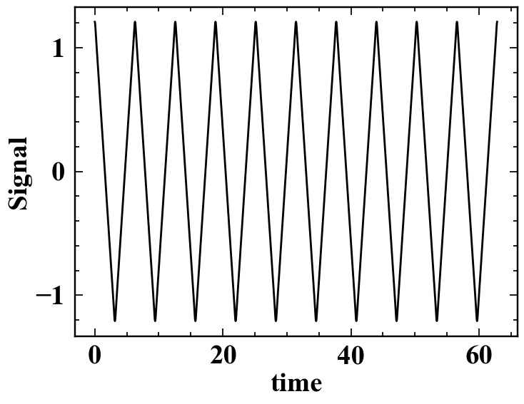
The data associated with this triangle wave is included in signal.dat, and the first ten lines will be outputted to the terminal with head:

$ head signal.dat

time                     signal
0.000000000000000000e+00 1.208721311121388364e+00
6.283185307179586614e-03 1.208524005375646748e+00
1.256637061435917323e-02 1.207933122945394233e+00
1.884955592153875897e-02 1.206951758516047635e+00
2.513274122871834645e-02 1.205585037553673411e+00
3.141592653589793394e-02 1.203840068169563127e+00
3.769911184307751795e-02 1.201725874483989820e+00
4.398229715025710196e-02 1.199253312231516322e+00
5.026548245743669291e-02 1.196434967546847306e+00

A Python file is already provided to compute the discrete Fourier transform of these data, and may be viewed carefully with nano or safely with the read-only pager less. The python file requires several modules including numpy and pylab, which are not accessible without appropriately modifying our environment. To demonstrate this, output the $PATH environment variable:

$ echo $PATH
$ which python

/home/rcsparky/.local/bin:/usr/local/bin:/usr/bin:/usr/local/sbin:/usr/sbin

/usr/bin/python

Note that this environment variable contains directories delimited by a colon character. These are the directories, or paths, that the shell searches for executables when given a command to run. That is, in the above example, the shell looks for an executable called echo first in ~rcsparky/.local/bin before checking /usr/local/bin, where the latter is where echo is first found. Python exists as an executable by default on Linux systems, as it is useful and often used for system administration. By running which python, the first instance of python as an executable within the specified $PATH is shown: /usr/bin/python. However, on Sol, the correct module file has to be loaded to properly set up the shell environment to access the correct scientific python. That is,

$ module load mamba/latest
$ echo $PATH
$ which python

=====================================================================
This module is intended solely for building or source activating user
python environments, i.e.,

    mamba create -n myenv -c conda-forge <package_list>

or

    source activate myenv

To list available environments, run:

    mamba info --envs

See our docs: https://links.asu.edu/solpy

Any other use is NOT TESTED.
=====================================================================

/packages/apps/mamba/1.2.0/bin:/home/rcsparky/.local/bin:/usr/local/bin:/usr/bin:/usr/local/sbin:/usr/sbin

/packages/apps/mamba/1.2.0/bin/python

When the mamba/latest module is loaded, among other background updates, the environment $PATH is updated so that a new python executable and its libraries are found by the shell first: /packages/apps/mamba/1.2.0/bin/python. However, this base environment should also not be used for computational research tasks. mamba is a python package manager that can be used to create custom python environments (see Sol’s documentation on mamba for details, which are beyond the scope of this shell lesson). When mamba/latest was module loaded, a help-text blurb was printed out which reflected that the module is intended solely for building or activating user python environments. The python environment scicomp is an administrator maintained, mamba-created software environment that may be used for common computational research tasks, such as reading or writing datafiles, or doing visualization.

$ source activate scicomp
(scicomp) $ echo $PATH
(scicomp) $ which python

/packages/envs/scicomp/bin:/packages/apps/mamba/1.2.0/condabin:/packages/apps/mamba/1.2.0/bin:/home/rcsparky/.local/bin:/usr/local/bin:/usr/bin:/usr/local/sbin:/usr/sbin

/packages/envs/scicomp/bin/python

Required steps to use python for computational research, in summary

1. Load the python package manager: module load mamba/latest
2. Activate the appropriate environment, e.g., source activate scicomp If the appropriate environment needs to be built, use mamba to create the environment and install all computational dependencies as detailed in our documentation. Note that when a python environment is source activated, the shell prompt is prefixed with the parenthetical name of that environment.

Module Environments

To see a list of loaded modules, use module list. To see all modules available on Sol, use module avail or refine your search to the software you are interested in by adding it as an additional argument, e.g., module avail matlab. To see more details about what a module actually does, try module show <name of module>.

So far, everything we have done has been on a head node, e.g., login01. The head node is provided mostly for managing compute rather than actively computing. On the head node, you are limited to a small set of actions, such as managing the file system, compiling software, or editing software. The main purpose of the node is to prepare, submit, and track work conducted through the SLURM scheduler. One of the simplest ways to actually get to a full compute environment is to use the system administrator provided command: interactive.

$ cd ~/Desktop/data-shell/signal
$ interactive -t 15

Note that the -t 15 option passed to interactive. This asks for a 15-minute allocation somewhere on the supercomputer. By default, interactive will request one core for four hours on one of Sol’s nodes within the general partition. To increase the likelihood of being immediately scheduled, we can decrease the time being asked for to something more practical, i.e., -t 15. Once the interactive job begins on a compute node, you will be automatically connected. Your prompt should reflect this, changing from [username@head_node_hostname:~/Desktop/data-shell/signal]$ to [username@compute_node_hostname:~/Desktop/data-shell/signal]$. In the above example, rcsparky was scheduled on c002. To explore this compute node, consider the following commands:

$ hostname # prints the compute node's hostname
$ nproc    # prints the number of processors (cores) available
$ free -h  # shows the amount of RAM available and its use on the node in
           # human readable format
$ pwd      # prints the working (current) directory
$ lscpu    # prints more detailed information about the cpu hardware

c002.sol.asu.edu 
1
              total        used        free      shared  buff/cache   available
Mem:          503Gi        13Gi       483Gi       2.7Gi       6.5Gi       484Gi
Swap:         4.0Gi       1.7Gi       2.3Gi
/home/rcsparky/Desktop/data-shell/signal
Architecture:        x86_64
CPU op-mode(s):      32-bit, 64-bit
Byte Order:          Little Endian
CPU(s):              128
On-line CPU(s) list: 0-127
Thread(s) per core:  1
Core(s) per socket:  64
Socket(s):           2
NUMA node(s):        8
Vendor ID:           AuthenticAMD
CPU family:          25
Model:               1
Model name:          AMD EPYC 7713 64-Core Processor
Stepping:            1
CPU MHz:             3093.695
BogoMIPS:            3992.37
Virtualization:      AMD-V
L1d cache:           32K
L1i cache:           32K
L2 cache:            512K
L3 cache:            32768K
NUMA node0 CPU(s):   0-15
NUMA node1 CPU(s):   16-31
NUMA node2 CPU(s):   32-47
NUMA node3 CPU(s):   48-63
NUMA node4 CPU(s):   64-79
NUMA node5 CPU(s):   80-95
NUMA node6 CPU(s):   96-111
NUMA node7 CPU(s):   112-127
Flags:               fpu vme de pse tsc msr pae mce cx8 apic sep mtrr
pge mca cmov pat pse36 clflush mmx fxsr sse sse2 ht syscall nx mmxext
fxsr_opt pdpe1gb rdtscp lm constant_tsc rep_good nopl nonstop_tsc cpuid
extd_apicid aperfmperf pni pclmulqdq monitor ssse3 fma cx16 pcid sse4_1
sse4_2 x2apic movbe popcnt aes xsave avx f16c rdrand lahf_lm cmp_legacy
svm extapic cr8_legacy abm sse4a misalignsse 3dnowprefetch osvw ibs
skinit wdt tce topoext perfctr_core perfctr_nb bpext perfctr_llc mwaitx
cpb cat_l3 cdp_l3 invpcid_single hw_pstate ssbd mba ibrs ibpb stibp
vmmcall fsgsbase bmi1 avx2 smep bmi2 invpcid cqm rdt_a rdseed adx smap
clflushopt clwb sha_ni xsaveopt xsavec xgetbv1 xsaves cqm_llc
cqm_occup_llc cqm_mbm_total cqm_mbm_local clzero irperf xsaveerptr
wbnoinvd amd_ppin arat npt lbrv svm_lock nrip_save tsc_scale vmcb_clean
flushbyasid decodeassists pausefilter pfthreshold v_vmsave_vmload vgif
v_spec_ctrl umip pku ospke vaes vpclmulqdq rdpid overflow_recov succor
smca sme sev sev_es

Lightwork

If you are planning on doing light interactive work, like compiling code or building a python environment, working on a homework problem, or developing/debugging a program, an alternative command aux-interactive will connect you to one of two dedicated lightwork nodes. These sessions are meant to always start quickly and by default ask for one core for one hour.

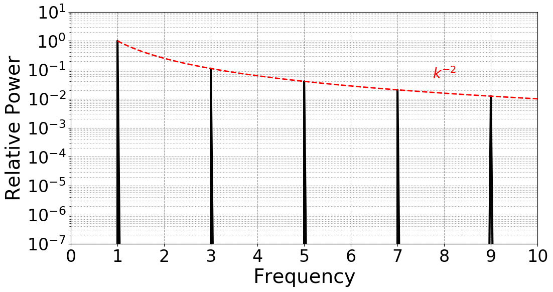
Let’s run the python fft script from this interactive session. All we need to do is set up the appropriate environment and run the script.

$ module load mamba/latest   # reset the environment 
$ python get_fft.py          # run the python code

The result is fft.png, demonstrating the expecting Fourier spectra of the triangle wave:

The interactive command

The command interactive is really a bash wrapper around SLURM’s provided scheduler command ,sbatch. On Sol, interactive has the following defaults:

• partition: general
• qos: public
• walltime: 0-4 (4 hours)
• cores: 1
• output: /dev/null (output messages are thrown away)
• error: /dev/null (error messages are thrown away) The defaults, as indicated, may be customized by passing the appropriate sbatch options. A full list may be obtained through the manual page: man sbatch, but a few common alternatives are indicated here:
• specify htc partition: -p htc
• specify public qos: -q public
• specify four hour wall time (max for this partition): -t 0-4 or -t 240 or many other ways
• specify four cores: -c 4
• specify one GPU: -G 1
• specify output file: -o <path>
• specify error file: -e <path> This will be examined in more detail in the sbatch section.

After a while of getting comfortable with interactive sessions, you may find yourself wishing there was a way to automate your actions. The good news is that your workflow is likely fully scriptable, and that it just requires a bit of scheduler wrapping to successful batch process. We will use the previous example to demonstrate with the file data-shell/signal/my_signal_processing_job.sh, which contains:

#!/bin/bash
#SBATCH -p general
#SBATCH -q public
#SBATCH -t 5
#SBATCH -c 1
#SBATCH -e signal_processing_job.%j.err
#SBATCH -o signal_processing_job.%j.out
#SBATCH --mail-type=ALL
#SBATCH --export=NONE

# Grab node information if desired (note a lot of this is recorded by
# slurm already)
echo hostname: $(hostname)
echo    nproc: $(nproc)
echo     free: $(free -h)
echo      pwd: $(pwd)
# Load required software
module load mamba/latest
source activate scicomp
# Diagnostic information
module list
which python
# Put bash into a diagnostic mode that prints commands
set -x
# Starting
echo STARTED: $(date)
# Run scientific workflow
python get_fft.py
# Finished
echo FINISHED: $(date)

To submit this job, use sbatch (submitted as user jyalim):

$ sbatch my_signal_processing_job.sh

Submitted batch job 9483816

The job id that sbatch reports is a unique integer associated with your job. This job id may be used to track the status of the job in the queue with a variety of commands, such as myjobs, a wrapper around the scheduler-provided program squeue that provides a filter for just your jobs:

$ myjobs

  JobID  PRIORITY     PARTITION/QOS  NAME                           STATE  TIME  TIME_LIMIT  Node/Core/GPU    NODELIST(REASON)
9483816     99693  lightwork/public  my_signal_processing_job.sh  PENDING  0:00        5:00  1/1/NA           (None)

or for more detailed information, thisjob <jobid>,

$ thisjob 9483427

JOBID      PARTITION NAME               USER           STATE        TIME         TIME_LIMIT   CPUS  NODELIST(REASON
9483816    lightwork my_signal_processi jyalim         PENDING      0:00         5:00         1     (None)

JobId=9483816 JobName=my_signal_processing_job.sh
   UserId=jyalim(513649) GroupId=grp_jyalim(99999988) MCS_label=N/A
   Priority=99693 Nice=0 Account=grp_jyalim QOS=public
   JobState=PENDING Reason=None Dependency=(null)
   Requeue=1 Restarts=0 BatchFlag=1 Reboot=0 ExitCode=0:0
   DerivedExitCode=0:0
   RunTime=00:00:00 TimeLimit=00:05:00 TimeMin=N/A
   SubmitTime=2023-08-22T17:39:00 EligibleTime=2023-08-22T17:39:00
   AccrueTime=Unknown
   StartTime=Unknown EndTime=Unknown Deadline=N/A
   SuspendTime=None SecsPreSuspend=0 LastSchedEval=2023-08-22T17:39:00 Scheduler=Main
   Partition=lightwork AllocNode:Sid=slurm01:2436840
   ReqNodeList=(null) ExcNodeList=cg00[1-5],fpga01a,fpga01i,g[230-239],g0[01-50]
   NodeList=
   NumNodes=1 NumCPUs=1 NumTasks=1 CPUs/Task=1 ReqB:S:C:T=0:0:*:*
   ReqTRES=cpu=1,mem=2G,node=1,billing=1
   AllocTRES=(null)
   Socks/Node=* NtasksPerN:B:S:C=0:0:*:* CoreSpec=*
   MinCPUsNode=1 MinMemoryCPU=2G MinTmpDiskNode=0
   Features=public DelayBoot=00:00:00
   OverSubscribe=YES Contiguous=0 Licenses=(null) Network=(null)
   Command=/home/jyalim/Desktop/data-shell/signal/my_signal_processing_job.sh
   WorkDir=/home/jyalim/Desktop/data-shell/signal
   StdErr=/home/jyalim/Desktop/data-shell/signal/signal_processing_job.9483816.err
   StdIn=/dev/null
   StdOut=/home/jyalim/Desktop/data-shell/signal/signal_processing_job.9483816.out
   Power=
   MailUser=jyalim@asu.edu MailType=INVALID_DEPEND,BEGIN,END,FAIL,REQUEUE,STAGE_OUT

Note that myjobs is roughly equivalent to squeue --me (the formatted outputs are different).

When scheduling jobs, it can be useful to gauge the activity on the supercomputer. The command-line program ns will provide a quick color-coded overview of partition status:

$ ns

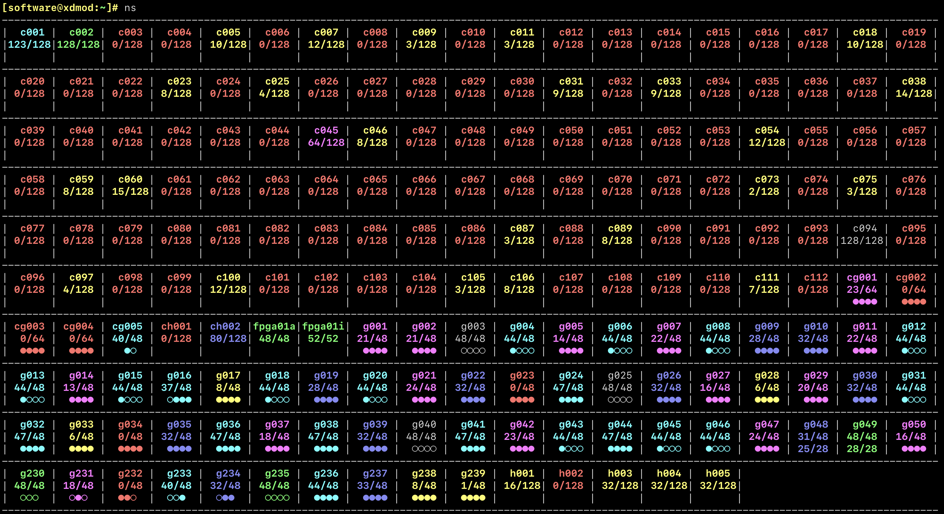
Green is used to indicate a full node is available within the partition, with varying colors reflective of varying availability or node status. For instance, red reflects that a node is fully allocated, whereas gray indicates that a node is offline. The first line in each box gives the short hostname of the node on the supercomputer, the second provides the number of cores that are allocated by the scheduler out of the system’s total cores, and the presence of a third line indicates GPU availability, using a ratio similar to the second line for our GPU-sliced nodes or empty (idle) and filled (allocated) circular symbols.

Another useful resource is the status page.

Cancelling jobs

The SLURM command scancel is one of the more important scheduler commands to know. In its simplest application, you may pass the job ids you would like to cancel, e.g. scancel 4967966. However, scancel can accept options to cancel all jobs associated with username, partitions, qos, state,and more. For instance, if issued by the user, scancel --me would cancel all jobs associated with that user. See man scancel for more details.

Job Efficiency

To better understand how your job is utilizing resources as it is running, you can use ssh to connect to allocated compute nodes and run programs like htop. This view will detail how much RAM or how many cores your jobs are utilizing (RES and CPU% columns in the process table). After a job has finished running, the scheduler can report on efficiency as well. Using seff <jobid> on a completed job will provide a simple summary of maximum RAM utilized relative to the amount requested as well as the amount of CPU utilized relative to number of cores requested. As Sol is a shared resource, it is important to keep your computational work as efficient as practically possible! Before submitting large batches of work, be sure to tune your allocations to best match your requirements!

Key Points

• The module system keeps the supercomputer environment adaptive to each researcher.

• Interactive sessions are useful for debugging or active job monitoring, e.g. htop.

• Using the scheduler to submit scripts through sbatch is an ultimate scaling goal

• Many commands are provided to aide the researcher, e.g. myjobs, ns, or interactive