Numeric Python (NumPy)
Last updated on 2024-12-05 | Edit this page
Overview
Questions
- How can I process tabular data files in Python?
Objectives
- Explain what a library is and what libraries are used for.
- Import a Python library and use the functions it contains.
- Read tabular data from a file into a program.
- Select individual values and subsections from data.
- Perform operations on arrays of data.
\(\newcommand{\coloneq}{\mathrel{≔}}\) \(\def\doubleunderline#1{\underline{\underline{#1}}}\) \(\def\tripleunderline#1{\underline{\doubleunderline{#1}}}\) \(\def\tprod{{\small \otimes}}\) \(\def\tensor#1{{\bf #1}}\) \(\def\mat#1{{\bf #1}}\) \(\renewcommand{\vec}[1]{{\bf #1}}\) \(\def\e{\vec{e}}\)
Words are useful, but what’s more useful are the sentences and stories we build with them. Similarly, while a lot of powerful, general tools are built into Python, specialized tools built up from these basic units live in libraries that can be called upon when needed.
The ndarray
The base work-horse of the NumPy framework is the
ndarray object. This object provides a performant container
for tensor algebra. Its performance, capabilities, base coverage, and
syntactical flavor are all based on the default array type from MATLAB,
but arguably provides greater flexibility for the programmer, especially
for third-order or larger tensors.
For those familiar with MATLAB, many syntactical features and operations will seem familiar, but there are subtle differences that may be awkward at first. For a full reference, see the official docs, NumPy for MATLAB users, which provides a Rosetta-Stone-like guide for MATLAB users.
The very first thing to do in Python to work with NumPy is to import the external library:
This line of code imports the external library into the workspace,
renaming it by common convention to np. The
as np is a shorthand that would have been equivalent to a
second line of code assigning the name np=numpy. For the
rest of this lesson, we will assume that NumPy has been
imported into the workspace as np. This only
has to be done once per Python invocation. Typically, it will be done at
the top of a Python script (in the header), or in the very first cell of
a Jupyter notebook.
To actually use the library — i.e., access the classes and methods
within it — we have to write np. and then the target
code.
OUTPUT
[0 1 2 3 4]
 `a` is of type: <class 'numpy.ndarray'>
 and `a[0]` type: <class 'numpy.int64'>
The code above prints the result of using the
numpy.arange method, which is similar to the built-in
range method, but in this instance instead generates a
one-dimensional ndarray object with the first five
non-negative integers (recall, Python is zero-indexed). Also, the
elements of the generated ndarray, a, are not
“vanilla” Python int objects. Instead they are 64-bit
integer objects provided by the NumPy library. This is an implicit hint
that we are using Python as a medium for all future computations: Python
is slow so we use it as a convienent interface
with fast NumPy to set up the data structures and communicate logical
instructions for data transformations.
Note that numpy.arange is an
overloaded function, meaning that we can pass
a floating-point argument to generate the appropriate NumPy
ndarray of numpy.float64 values very
easily.
OUTPUT
[0. 1. 2. 3. 4.]
 `x` is of type: <class 'numpy.ndarray'>
 and `x[0]` type: <class 'numpy.float64'>
This is a valid use of the numpy.arange method, but
typically we will want to only generate ranges of
numpy.int64 with the method. The rest of the materials will
only use the arange method for generating integer
ndarrays.
Unlike the built-in list, the NumPy ndarray
automatically broadcasts scalar arithmetic to
the elements of the ndarray:
OUTPUT
1+a: [1 2 3 4 5]
2*a: [0 2 4 6 8]
For MATLAB users,
np.arange(<start>,<excluded end>,<stride>)
provides functionality like the colon operator,
<start>:<stride>:<included end>. Thus, we
may generate an ndarray of odd numbers without list
comprehension, improving performance as a perk,
PYTHON
# benchmark generating the first ten-million odds with vanilla Python
# NOTE: `%timeit` is a "Jupyter Magic," a Jupyter macro, not Python!
%timeit odd_list = [2*k+1 for k in range(10**7)]
%timeit odd_list2 = [k for k in range(1,2*10**7,2)]
%timeit odd_list3 = list(range(1,2*10**7,2))
OUTPUT
393 ms ± 884 µs per loop (mean ± std. dev. of 7 runs, 1 loop each)
198 ms ± 544 µs per loop (mean ± std. dev. of 7 runs, 10 loops each)
148 ms ± 207 µs per loop (mean ± std. dev. of 7 runs, 10 loops each)
PYTHON
# benchmark generating the first ten-million odds with NumPy
%timeit odd_array = 2*np.arange(10**7)+1
# Even less Python and more NumPy:
%timeit odd_array2 = np.arange(1,2*10**7,2)
OUTPUT
13 ms ± 550 µs per loop (mean ± std. dev. of 7 runs, 100 loops each)
8 ms ± 90 µs per loop (mean ± std. dev. of 7 runs, 100 loops each)
Vanilla Python is, at best and worst, nearly 20–50 times slower than NumPy! Why is this? It may help to spell out the operations involved.
Vanilla Python
In this approach, Python is asked to do ten-million product and sum
operations (twenty-million actions), and store the results in a generic,
unoptimized list object. The second attempt redundantly
converts the generated iterates of range(1,2*10**7,2) to a
list, improving performance by a factor of two. The final attempt
removes the redundant list comprehension.
First NumPy approach
In this solution, odd_array = 2*np.arange(10**7)+1,
NumPy is asked to generate a list of the first ten-million non-negative
integers, which is done in a performant C library with the updated
memory accessible from Python’s workspace. Then NumPy is told — through
broadcasting — to multiply every element by two and add one. It’s still
twenty-million actions, but the difference is that Python is only
involved up to three times; the rest is done in an expertly written
backend library which is nearly 30 times faster than the comparable
approach in vanilla Python.
Naive matrix multiplication
This next example would have been counter productive to introduce prior to NumPy, as it is an exhausting exercise to even generate two-dimensional lists in vanilla Python. However, it’s much simpler with NumPy. For instance, to generate a four-by-four of uniformly random numbers in \((0,1)\):
OUTPUT
[[0.95781959 0.9915284  0.58248825 0.41600528]
 [0.77493045 0.67522185 0.00530085 0.2539285 ]
 [0.53248467 0.75761823 0.69219508 0.58811258]
 [0.59892653 0.77743011 0.95975933 0.71425297]]
Or we would have to use the standard random library,
which encourages bad habits (technique with Python lists and
random that should not be practiced, although nested list
comprehension has its place in the toolbox):
PYTHON
import random
A = [ [random.random() for column in range(4)] for row in range(4) ]
for row in A: print(row)
OUTPUT
[0.6818582562400426, 0.6868889674612016, 0.34483486515037653, 0.9638090861458387]
[0.24086075915520622, 0.07221778821332858, 0.43624157264612706, 0.7935877715986276]
[0.6585256801337919, 0.2631377880223672, 0.9586513851146543, 0.9070537970347129]
[0.1566693962998439, 0.8860807403362514, 0.039423876906426014, 0.44815646838680734]
We will write a few functions to do matrix multiplication with vanilla Python.
PYTHON
def vanilla_dot_product(u,v):
    running_sum = 0
    for i in range(len(u)):
        running_sum += u[i]*v[i]
    return running_sum
def vanilla_matrix_vector_product(A,x):
    y = [ vanilla_dot_product(a,x) for a in A ]
    return y
def vanilla_matrix_tranpose(A):
    # `*A` passes the first-elements of `A` --- the rows --- to zip as
    # arguments, as if we wrote every row of `A` explicitly.
    # `zip` is a built-in function that iteratively combines the first
    # elements of its arguments, allowing us to iterate over the cols of
    # `A`.
    # `map` is a built-in function that shortcuts a for loop: we are
    # mapping every column of `A` to the `list` class, converting the
    # immutable tuples to lists.
    # The final `list` ensures that `A_Transposed` is a two-dimensional
    # container of "column vectors."
    A_Tranposed = list(map(list,zip(*A)))
    return A_Tranposed
def vanilla_matrix_matrix_product(A,B):
    # `*B` passes the first-elements of `B` --- the rows --- to zip as
    # arguments, as if we wrote every row of `B` explicitly.
    # `zip` is a built-in function that iteratively combines the first
    # elements of its arguments, allowing us to iterate over the cols of
    # `B`.
    CT = [ vanilla_matrix_vector_product(A,b_col) for b_col in zip(*B) ]
    C  = vanilla_matrix_tranpose(CT)
    return C
PYTHON
# originally 1000x1000, but list method takes way too long
A,B = np.random.rand(2,100,100)
AL,BL = A.tolist(),B.tolist()
%timeit CL = vanilla_matrix_matrix_product(AL,BL)
# A@B implicitly calls LAPACK dgemm and parallelizes if multiple cores
%timeit C = A@B
# Validate accuracy of custom matrix-matrix product
CL = vanilla_matrix_matrix_product(AL,BL)
C  = A@B
# compute elementwise error matrix
elementwise_error = C - np.array(CL)
# print out the Frobenius norm of the error matrix
print(f'Fro. norm: {np.linalg.norm(elementwise_error)}')
# Another way to check
print(f'Are all elements close? {np.all(np.isclose(C,np.array(CL)))}')
OUTPUT
22.5 ms ± 58.7 µs per loop (mean ± std. dev. of 7 runs, 10 loops each)
303 µs ± 15.5 µs per loop (mean ± std. dev. of 7 runs, 1,000 loops each)
Fro. norm: 2.3464053421603193e-13
Are all elements close? True
The simpler matrix-matrix product provided by NumPy, by just using
the @ operator for the two matrices, is nearly 65 times
faster than the vanilla approach, and will automatically use multiple
cores for us.
Approximating derivatives
The second-order, central finite difference stencil, \[\dfrac{u(x_{i+1})-u(x_{i-1})}{2\Delta x},\] where \(\Delta x=x_1-x_0\) is the uniform spatial step, approximates the first derivative of a function \(u\) at a point \(x_i\). Let \(u(x)=\sin(x)\) for \(x\in[0,2\pi)\) and discretize the domain such that \(x_i = 2\pi i/N\) for \(i=0,...,N\). Use NumPy matrix multiplication to compute the first derivative of \(u\) with \(N=10^k\) for \(k=1,...,4\), by constructing the appropriate dense operator \(D\) for the stencil. Using a 2-norm, how does the error change with \(\Delta x\)?
Extra Credit: since the stencil is very sparse, how could we improve the performance of the code and go to larger \(N\)? What is the largest \(N\) we could go to, and why?
The discretization of the domain together with the periodicity of \(u\) and the second-order stencil induces a set of linear equations, \[D_{ij}u_j \approx u_j',\] \[ \dfrac{1}{2\Delta x} \begin{bmatrix} 0 & 1 & 0 & ... & 0 & -1 \\ -1 & 0 & 1 & 0 & & 0 \\ 0 & -1 & 0 & \ddots &\ddots& \vdots\\ \vdots & 0 & \ddots & \ddots & 1 & 0 \\ 0 & & \ddots & -1 & 0 & 1 \\ 1 & 0 & ... & 0 & -1 & 0 \\ \end{bmatrix} \begin{bmatrix} u(x_0) \\ u(x_1) \\ \vdots \\ u(x_{N-3}) \\ u(x_{N-2}) \\ u(x_{N-1}) \\ \end{bmatrix} \approx \begin{bmatrix} u'(x_0) \\ u'(x_1) \\ \vdots \\ u'(x_{N-3}) \\ u'(x_{N-2}) \\ u'(x_{N-1}) \\ \end{bmatrix}, \] where \(D\in\mathbb{R}^{N\times N}\).
The following code defines a function, challenge, which
takes an input \(N\) and computes the
relative error. It also plots the degree of error on a log.-log. scale,
demonstrating that the stencil’s truncation error converges to the
analytical solution quadratically with the step size, \(\Delta x\).
PYTHON
import numpy as np
import matplotlib.pyplot as plt
def challenge(N):
    # N+1 is important here, because definition of x
    x = np.linspace(0,2*np.pi,N+1)[:-1]
    dx= x[1]-x[0]
    u = np.sin(x)
    # put 1 and -1 on super- and sub-diagonal, respectively
    D = np.diag(np.ones(N-1),1)-np.diag(np.ones(N-1),-1)
    # circulant derivative operator (periodicity)
    D[0,-1] =-1
    D[-1,0] = 1
    D /= 2*dx
    # compute derivative
    du= D@u
    # exact result
    ex= np.cos(x)
    rel_err = np.linalg.norm(ex-du)/np.linalg.norm(ex)
    return rel_err

Ns = 10**np.arange(1,5)
rel_errs = np.array([challenge(N) for N in Ns])
dxs = 2*np.pi / Ns
plt.loglog(dxs,rel_errs,'ro-',linewidth=2,label='Relative Error')
c = np.polyfit(np.log(dxs),np.log(rel_errs),1)
h = np.logspace(-4,0,41)
E = np.exp(c[1])*h**c[0]
plt.loglog(h,E,'k-',linewidth=3,zorder=-1,label='Algebraic Fit')
plt.legend()
print(f'Relative error is second order in ∆x: {c[0]:.5f}')
OUTPUT
Relative error is second order in ∆x: 1.99742
Discussion
The above approach worked well for \(N\) up to \(10^4\). What would happen in \(N\) were increased much further for the same system? The size of \(D\) grows like \(N^2\), so very quickly we’ll run out of fast CPU memory, called “cache,” and likely run out of RAM too, causing out-of-memory errors.
The stencil in the challenge results in an extremely sparse operator representation for \(D\). Thus, using a dense representation is extremely inefficient, regardless of the performant backend. A better solution code then could have
- used sparse matrices instead of a dense one,
- used index slicing to represent the operations,
- or probably the fastest: used the
np.rollinstead to account for the periodicity.
Demonstrating this last point:
du = (np.roll(u,-1)-np.roll(u,+1))/(2*dx) allows for a much
faster approximation of order \(N\)
instead of \(N^2\).
However, for \(N\) beyond \(10^6\), the error will begin to increase as rounding errors begin to dominate the total error of the approximation.
Attributes of ndarray instances
Jupyter Tips and Tricks
To see all the possible methods and attributes under a workspace
name, like a as defined by
a=np.linspace(0,1,5), use the Tab key after
typing a dot. I.e., typing a+.+Tab will
show a context menu of all possible sub-names to complete for that
object, a.
NumPy’s ndarray class provides its instances with a
variety of rich methods. These methods allow for syntactically sweet
data transformation. We highlight a few of the common methods below.
PYTHON
# generate an `ndarray` over [0,1] with 5 points with uniform spacing,
# such that $x_k=a+k(b-a)/(N-1)$ for $k\in[0,N)\subset\mathbb{Z}$.
a,b,N = 0,1,5
x = np.linspace(a,b,N)
print(f'`x`: {x}\n`x*x`: {x*x}\n`x@x`: {x@x}')
# print a horizontal rule 72-characters long with " x " centered
print(f'{" x ":=^72}')
# summary characteristics for x:
x_min, x_mean, x_max, x_std = x.min(), x.mean(), x.max(), x.std()
print(f'min: {x_min}\nmean: {x_mean}\nmax: {x_max}\nstandard dev.: {x_std}')
x_sum, x_shape, x_transpose = x.sum(), x.shape, x.T
print(f'sum: {x_sum}\nshape: {x_shape}\ntranspose: {x_transpose}')
OUTPUT
`x`: [0.   0.25 0.5  0.75 1.  ]
`x*x`: [0.     0.0625 0.25   0.5625 1.    ]
`x@x`: 1.875
================================== x ===================================
min: 0.0
mean: 0.5
max: 1.0
standard dev.: 0.3535533905932738
sum: 2.5
shape: (5,)
transpose: [0.   0.25 0.5  0.75 1.  ]
Note that these object methods are also functions at NumPy’s root.
For instance, instead of x.min() we could have equivalently
run np.min(x). One reason to do the latter instead of the
former is if we are potentially mixing object types as inputs —
np.min(L) will work when L is a list object,
but then L.min() is undefined. For new and expert users, a
good practice is to use the object’s method calls (x.min())
as it is faster to write and encourages the use of performant
ndarray objects over lists for numerical data.
However, not everything is defined as a method call. For instance,
the median must be computed with np.median. Additionally,
the convenience attribute .T is not a method call, but an
attribute, which returns a view of the
ndarray transposed. Note from the example that
x is truly one-dimensional with five elements and thus
x is equivalent to x.T. We did not have to
worry about the formal linear algebra rules for computing the squared
2-norm of x with x@x — NumPy was able to infer
that we meant to compute the inner product without adding a redundant
second dimension — or axis — to
x.
Linear algebra with NumPy
In this section, we will use some tensor algebra to make the operations more clear, as well as to introduce Einstein summation notation, which will allow us to use a very powerful NumPy tool later.
In tensor algebra, tensors are represented with linear combinations of basis tensors. For instance, for a simple three-dimensional vector, \(\vec{u}\), and a set of Euclidean unit vectors, \(\e_k\),
\[ \vec{u} = \begin{bmatrix}u_1\\u_2\\u_3\end{bmatrix} = u_1 \begin{bmatrix}1\\0\\0\end{bmatrix} + u_2 \begin{bmatrix}0\\1\\0\end{bmatrix} + u_3 \begin{bmatrix}0\\0\\1\end{bmatrix} = u_1 \e_1 + u_2 \e_2 + u_3 \e_3 = \sum_{k=1}^3 u_k \e_k. \]
The Cartesian outer products of Euclidean unit vectors form a natural basis for representing matrices:
\[ \mat{A} = \begin{bmatrix}A_{11}&A_{12}\\A_{21}&A_{22}\\\end{bmatrix} = A_{11} \begin{bmatrix}1&0\\0&0\\\end{bmatrix} + A_{12} \begin{bmatrix}0&1\\0&0\\\end{bmatrix} + A_{21} \begin{bmatrix}0&0\\1&0\\\end{bmatrix} + A_{22} \begin{bmatrix}0&0\\0&1\\\end{bmatrix} \\ = \sum_{j=1}^2\sum_{k=1}^2 A_{jk} \e_j \e_k^T \\ = \sum_{j=1}^2\sum_{k=1}^2 A_{jk} \e_j \tprod \e_k. \]
The notation \(\tprod\) refers to the tensor product that becomes necessary for representing higher-order tensors.
Tensor-tensor calculations then involve carrying out products of sums. For instance, an inner product of two \(\mathbb{R}^2\) vectors:
\[ \vec{u}^T\vec{v} = \left( \sum_{j=1}^2 u_j\e_j \right)^T \sum_{k=1}^2 v_k\vec{e_k} \\ = u_1 v_1 \e_1^T\e_1 + u_1 v_2 \e_1^T\e_2 + u_2 v_1 \e_2^T\e_1 + u_2 v_2 \e_2^T\e_2 \\ = \sum_{j=1}^2\sum_{k=1}^2 u_j v_k\e_j^T\e_k = \sum_{j=1}^2\sum_{k=1}^2 u_j v_k \delta_{jk} = \sum_{j=1}^2 u_j v_j = u_1 v_1 + u_2 v_2, \]
where \(\delta_{jk}\) is the Kronecker delta, which is zero unless \(j=k\), in which case it’s one [thanks to using a(n) (orthonormal) basis].
Einstein Summation Notation
Einstein summation notation is a more compact representation of tensor algebra, that simply drops the summation symbols. Continuing from the matrix example above, \(\mat{A}= A_{jk}\e_j\tprod \e_k\).
The inner product example also reduces to \(\vec{u}\cdot\vec{v}=u_j v_k \e_j\cdot\e_k = u_j v_j\).
D.1.1: One-dimensional ndarray operations
For this sub-section, define the following one-dimensional NumPy
ndarrays and variables:
\[ \texttt{N} \coloneq 5, \\ \textrm{Let: } k\in[0,N)\subset\mathbb{Z}, \\ \texttt{x} \coloneq \vec{x} = \frac{k}{N-1} \e_k, \\ \texttt{a} \coloneq \vec{a} = k \e_k. \]
OUTPUT
x: [0.   0.25 0.5  0.75 1.  ]
a: [0 1 2 3 4]
D.1.1.a elementwise operations
\[\texttt{x+a}\coloneq\vec{x}+\vec{a}= (x_i+a_i) \e_i\]
\[\texttt{x*a}\coloneq\vec{x}\odot\vec{a}= x_i a_i \e_i\]
OUTPUT
x+a: [0.   1.25 2.5  3.75 5.  ]
x*a: [0. 0.25 1. 2.25 4. ]D.1.1.c outer products
\[ \texttt{np.outer(x,a)} \coloneq \vec{x}\tprod\vec{a} =x_i a_j \e_i\tprod\e_j \]
\[ \texttt{np.add.outer(x,a)} \coloneq \vec{x}\tprod\vec{1}+\vec{1}\tprod\vec{a} = (x_i + a_j)\,\, \e_i\tprod\e_j, \]
where \(\vec{1}\) is a vector of all ones.
PYTHON
print(f'vector outer(x,a): (x_i*a_j)e_i e_j\n{np.outer(x,a)}\n')
print(f'addition outer(x,a): (x_i+a_j)e_i e_j\n{np.add.outer(x,a)}\n')
OUTPUT
vector outer(x,a): (x_i*a_j) e_i e_j
[[0.   0.   0.   0.   0.  ]
 [0.   0.25 0.5  0.75 1.  ]
 [0.   0.5  1.   1.5  2.  ]
 [0.   0.75 1.5  2.25 3.  ]
 [0.   1.   2.   3.   4.  ]]

addition outer(x,a): (x_i+a_j) e_i e_j
[[0.   1.   2.   3.   4.  ]
 [0.25 1.25 2.25 3.25 4.25]
 [0.5  1.5  2.5  3.5  4.5 ]
 [0.75 1.75 2.75 3.75 4.75]
 [1.   2.   3.   4.   5.  ]]
D.2.1 Matrix-vector operations
For this sub-section, define the following one- and two-dimensional
NumPy ndarrays and variables:
\[ \texttt{N} \coloneq N=4, \\ \textrm{Let: } k\in[0,N^2)\subset\mathbb{Z}, \quad \mu=\Bigl\lfloor \frac{k}{N}\Bigr\rfloor, \quad \nu= k \bmod N \\ \texttt{A} \coloneq \mat{A} = k^2\,\, \e_\mu \tprod \e_\nu. \\ \textrm{Let: } j\in[0,N)\subset\mathbb{Z}, \\ \texttt{x} \coloneq \vec{x} = (j+1)\,\,\e_j. \]
OUTPUT
A:
 [[  0   1   4   9]
 [ 16  25  36  49]
 [ 64  81 100 121]
 [144 169 196 225]]

x: [1 2 3 4]
D.2.1.a Elementwise
Let \(i,j,k\in[0,N)\subset\mathbb{Z}\).
\[ \texttt{A+x} \coloneq \mat{A} + (\vec{1}\tprod \vec{x}) = (A_{ij}+x_j)\,\e_i\tprod\e_j \]
\[ \texttt{A*x} \coloneq \mat{A} \odot (\vec{1}\tprod \vec{x}) = (A_{ij} x_j)\,\e_i\tprod\e_j \]
OUTPUT
ELEMENTWISE BROADCASTING
        A+x
[[  1   3   7  13]
 [ 17  27  39  53]
 [ 65  83 103 125]
 [145 171 199 229]]

        A*x
[[  0   2  12  36]
 [ 16  50 108 196]
 [ 64 162 300 484]
 [144 338 588 900]]
D.2.1.b Matrix-vector operations
Let \(i,j\in[0,N)\subset\mathbb{Z}\).
\[ \texttt{x@A} \coloneq \vec{x}^T \mat{A} = A_{ij} x_i \e_j^T \]
\[ \texttt{A@x} \coloneq \mat{A} \vec{x} = A_{ij} x_j \e_i \]
OUTPUT
x@A
[ 800  970 1160 1370]

A@x
[  50  370 1010 1970]
D.2.1.c Solving \(\mat{A}\vec{x}=\vec{b}\)
Let \(i,j\in[0,N)\subset\mathbb{Z}\) and let \(\vec{b} = \mat{A}\vec{x}\). Then \(\vec{x}=A^{-1}_{ij}b_j\e_i\).
D.2.1.c.i Matrix inversion (bad)
PYTHON
b = A@x
A_inverse = np.linalg.inv(A)
x_approx  = A_inverse@b
print('Rel. Err.: ',np.linalg.norm(x_approx-x)/np.linalg.norm(x))
OUTPUT
Rel. Err.: 2.294921930407801D.2.1.c.ii Implicit solve (good)
PYTHON
b = A@x
x_approx  = np.linalg.solve(A,b)
print('Rel. Err.: ',np.linalg.norm(x_approx-x)/np.linalg.norm(x))
OUTPUT
Rel. Err.: 0.012225D.2.1.c.iii PLU solve (good, equivalent to previous)
PYTHON
import scipy
b = A@x
LU_and_pivots = scipy.linalg.lu_factor(A)
x_approx  = scipy.linalg.lu_solve(LU_and_pivots,b)
print('Rel. Err.: ',np.linalg.norm(x_approx-x)/np.linalg.norm(x))
OUTPUT
Rel. Err.: 0.012225D.2.1.c.iv Eig solve (worse)
PYTHON
b = A@x
evals,evecs = np.linalg.eig(A)
x_approx = evecs @ (np.linalg.solve(evecs,b)/evals)
print('Rel. Err.: ',np.linalg.norm(x_approx-x)/np.linalg.norm(x))
OUTPUT
Rel. Err.: 16.3456D.2.2 Matrix-matrix operations
For this sub-section, define the following two-dimensional NumPy
ndarrays and variables:
\[ \texttt{N} \coloneq N=2, \\ \textrm{Let: } k\in[0,N^2)\subset\mathbb{Z}, \quad \mu=\Bigl\lfloor \frac{k}{N}\Bigr\rfloor, \quad \nu= k \bmod N \\ \texttt{A} \coloneq \mat{A} = k^2\,\, \e_\mu \tprod \e_\nu \\ \texttt{B} \coloneq \mat{B} = k\,\, \e_\mu \tprod \e_\nu \]
PYTHON
N = 2
A = np.arange(N**2).reshape((N,N))**2
B = np.arange(N**2).reshape((N,N))
print(f'A:\n {A}\n\nB:\n {B}')
OUTPUT
A:
 [[0 1]
 [4 9]]

B:
 [[0 1]
 [2 3]]
D.2.2.a elementwise
Let \(i,j\in[0,N)\subset\mathbb{Z}\).
\[ \texttt{A+B} \coloneq \mat{A} + \mat{B} = (A_{ij} + B_{ij}) \,\, \e_i\tprod\e_j \]
\[ \texttt{A*B} \coloneq \mat{A} \odot \mat{B} = A_{ij} B_{ij} \,\, \e_i\tprod\e_j \]
OUTPUT
ELEMENTWISE BROADCASTING
   A+B
[[ 0  2]
 [ 6 12]]

   A*B
[[ 0  1]
[ 8 27]]Using ndarray built-in methods
Basic signal processing
Loading data into Python
To begin processing the clinical trial inflammation data, we need to load it into Python. We can do that using a library called NumPy, which stands for Numerical Python. In general, you should use this library when you want to do fancy things with lots of numbers, especially if you have matrices or arrays. To tell Python that we’d like to start using NumPy, we need to import it:
Importing a library is like getting a piece of lab equipment out of a storage locker and setting it up on the bench. Libraries provide additional functionality to the basic Python package, much like a new piece of equipment adds functionality to a lab space. Just like in the lab, importing too many libraries can sometimes complicate and slow down your programs - so we only import what we need for each program.
Once we’ve imported the library, we can ask the library to read our data file for us:
OUTPUT
array([[ 0.,  0.,  1., ...,  3.,  0.,  0.],
       [ 0.,  1.,  2., ...,  1.,  0.,  1.],
       [ 0.,  1.,  1., ...,  2.,  1.,  1.],
       ...,
       [ 0.,  1.,  1., ...,  1.,  1.,  1.],
       [ 0.,  0.,  0., ...,  0.,  2.,  0.],
       [ 0.,  0.,  1., ...,  1.,  1.,  0.]])
The expression numpy.loadtxt(...) is a function call that asks Python
to run the function
loadtxt which belongs to the numpy library.
The dot notation in Python is used most of all as an object
attribute/property specifier or for invoking its method.
object.property will give you the object.property value,
object_name.method() will invoke on object_name method.
As an example, John Smith is the John that belongs to the Smith
family. We could use the dot notation to write his name
smith.john, just as loadtxt is a function that
belongs to the numpy library.
numpy.loadtxt has two parameters: the name of the file we
want to read and the delimiter
that separates values on a line. These both need to be character strings
(or strings for short), so we put
them in quotes.
Since we haven’t told it to do anything else with the function’s
output, the notebook displays it.
In this case, that output is the data we just loaded. By default, only a
few rows and columns are shown (with ... to omit elements
when displaying big arrays). Note that, to save space when displaying
NumPy arrays, Python does not show us trailing zeros, so
1.0 becomes 1..
Our call to numpy.loadtxt read our file but didn’t save
the data in memory. To do that, we need to assign the array to a
variable. In a similar manner to how we assign a single value to a
variable, we can also assign an array of values to a variable using the
same syntax. Let’s re-run numpy.loadtxt and save the
returned data:
This statement doesn’t produce any output because we’ve assigned the
output to the variable data. If we want to check that the
data have been loaded, we can print the variable’s value:
OUTPUT
[[ 0.  0.  1. ...,  3.  0.  0.]
 [ 0.  1.  2. ...,  1.  0.  1.]
 [ 0.  1.  1. ...,  2.  1.  1.]
 ...,
 [ 0.  1.  1. ...,  1.  1.  1.]
 [ 0.  0.  0. ...,  0.  2.  0.]
 [ 0.  0.  1. ...,  1.  1.  0.]]
Now that the data are in memory, we can manipulate them. First, let’s
ask what type of thing
data refers to:
OUTPUT
<class 'numpy.ndarray'>The output tells us that data currently refers to an
N-dimensional array, the functionality for which is provided by the
NumPy library. These data correspond to arthritis patients’
inflammation. The rows are the individual patients, and the columns are
their daily inflammation measurements.
Data Type
A NumPy array contains one or more elements of the same type. The
type function will only tell you that a variable is a NumPy
array but won’t tell you the type of thing inside the array. We can find
out the type of the data contained in the NumPy array.
OUTPUT
float64This tells us that the NumPy array’s elements are floating-point numbers.
With the following command, we can see the array’s shape:
OUTPUT
(60, 40)The output tells us that the data array variable
contains 60 rows and 40 columns. When we created the variable
data to store our arthritis data, we did not only create
the array; we also created information about the array, called members or attributes. This extra
information describes data in the same way an adjective
describes a noun. data.shape is an attribute of
data which describes the dimensions of data.
We use the same dotted notation for the attributes of variables that we
use for the functions in libraries because they have the same
part-and-whole relationship.
If we want to get a single number from the array, we must provide an index in square brackets after the variable name, just as we do in math when referring to an element of a matrix. Our inflammation data has two dimensions, so we will need to use two indices to refer to one specific value:
OUTPUT
first value in data: 0.0OUTPUT
middle value in data: 16.0The expression data[29, 19] accesses the element at row
30, column 20. While this expression may not surprise you,
data[0, 0] might. Programming languages like Fortran,
MATLAB and R start counting at 1 because that’s what human beings have
done for thousands of years. Languages in the C family (including C++,
Java, Perl, and Python) count from 0 because it represents an offset
from the first value in the array (the second value is offset by one
index from the first value). This is closer to the way that computers
represent arrays (if you are interested in the historical reasons behind
counting indices from zero, you can read Mike
Hoye’s blog post). As a result, if we have an M×N array in Python,
its indices go from 0 to M-1 on the first axis and 0 to N-1 on the
second. It takes a bit of getting used to, but one way to remember the
rule is that the index is how many steps we have to take from the start
to get the item we want.
!['data' is a 3 by 3 numpy array containing row 0: ['A', 'B', 'C'], row 1: ['D', 'E', 'F'], androw 2: ['G', 'H', 'I']. Starting in the upper left hand corner, data[0, 0] = 'A', data[0, 1] = 'B',data[0, 2] = 'C', data[1, 0] = 'D', data[1, 1] = 'E', data[1, 2] = 'F', data[2, 0] = 'G',data[2, 1] = 'H', and data[2, 2] = 'I', in the bottom right hand corner.](fig/python-zero-index.svg)
In the Corner
What may also surprise you is that when Python displays an array, it
shows the element with index [0, 0] in the upper left
corner rather than the lower left. This is consistent with the way
mathematicians draw matrices but different from the Cartesian
coordinates. The indices are (row, column) instead of (column, row) for
the same reason, which can be confusing when plotting data.
Slicing data
An index like [30, 20] selects a single element of an
array, but we can select whole sections as well. For example, we can
select the first ten days (columns) of values for the first four
patients (rows) like this:
OUTPUT
[[ 0.  0.  1.  3.  1.  2.  4.  7.  8.  3.]
 [ 0.  1.  2.  1.  2.  1.  3.  2.  2.  6.]
 [ 0.  1.  1.  3.  3.  2.  6.  2.  5.  9.]
 [ 0.  0.  2.  0.  4.  2.  2.  1.  6.  7.]]
The slice 0:4 means,
“Start at index 0 and go up to, but not including, index 4”. Again, the
up-to-but-not-including takes a bit of getting used to, but the rule is
that the difference between the upper and lower bounds is the number of
values in the slice.
We don’t have to start slices at 0:
OUTPUT
[[ 0.  0.  1.  2.  2.  4.  2.  1.  6.  4.]
 [ 0.  0.  2.  2.  4.  2.  2.  5.  5.  8.]
 [ 0.  0.  1.  2.  3.  1.  2.  3.  5.  3.]
 [ 0.  0.  0.  3.  1.  5.  6.  5.  5.  8.]
 [ 0.  1.  1.  2.  1.  3.  5.  3.  5.  8.]]
We also don’t have to include the upper and lower bound on the slice. If we don’t include the lower bound, Python uses 0 by default; if we don’t include the upper, the slice runs to the end of the axis, and if we don’t include either (i.e., if we use ‘:’ on its own), the slice includes everything:
The above example selects rows 0 through 2 and columns 36 through to the end of the array.
OUTPUT
small is:
[[ 2.  3.  0.  0.]
 [ 1.  1.  0.  1.]
 [ 2.  2.  1.  1.]]
Analyzing data
NumPy has several useful functions that take an array as input to
perform operations on its values. If we want to find the average
inflammation for all patients on all days, for example, we can ask NumPy
to compute data’s mean value:
OUTPUT
6.14875mean is a function
that takes an array as an argument.
Not All Functions Have Input
Generally, a function uses inputs to produce outputs. However, some functions produce outputs without needing any input. For example, checking the current time doesn’t require any input.
OUTPUT
Sat Mar 26 13:07:33 2016For functions that don’t take in any arguments, we still need
parentheses (()) to tell Python to go and do something for
us.
Let’s use three other NumPy functions to get some descriptive values about the dataset. We’ll also use multiple assignment, a convenient Python feature that will enable us to do this all in one line.
PYTHON
maxval, minval, stdval = numpy.amax(data), numpy.amin(data), numpy.std(data)

print('maximum inflammation:', maxval)
print('minimum inflammation:', minval)
print('standard deviation:', stdval)
Here we’ve assigned the return value from
numpy.amax(data) to the variable maxval, the
value from numpy.amin(data) to minval, and so
on.
OUTPUT
maximum inflammation: 20.0
minimum inflammation: 0.0
standard deviation: 4.61383319712Mystery Functions in IPython
How did we know what functions NumPy has and how to use them? If you
are working in IPython or in a Jupyter Notebook, there is an easy way to
find out. If you type the name of something followed by a dot, then you
can use tab completion
(e.g. type numpy. and then press Tab) to see a
list of all functions and attributes that you can use. After selecting
one, you can also add a question mark
(e.g. numpy.cumprod?), and IPython will return an
explanation of the method! This is the same as doing
help(numpy.cumprod). Similarly, if you are using the “plain
vanilla” Python interpreter, you can type numpy. and press
the Tab key twice for a listing of what is available. You can
then use the help() function to see an explanation of the
function you’re interested in, for example:
help(numpy.cumprod).
Confusing Function Names
One might wonder why the functions are called amax and
amin and not max and min or why
the other is called mean and not amean. The
package numpy does provide functions max and
min that are fully equivalent to amax and
amin, but they share a name with standard library functions
max and min that come with Python itself.
Referring to the functions like we did above, that is
numpy.max for example, does not cause problems, but there
are other ways to refer to them that could. In addition, text editors
might highlight (color) these functions like standard library function,
even though they belong to NumPy, which can be confusing and lead to
errors. Since there is no function called mean in the
standard library, there is no function called amean.
When analyzing data, though, we often want to look at variations in statistical values, such as the maximum inflammation per patient or the average inflammation per day. One way to do this is to create a new temporary array of the data we want, then ask it to do the calculation:
PYTHON
patient_0 = data[0, :] # 0 on the first axis (rows), everything on the second (columns)
print('maximum inflammation for patient 0:', numpy.amax(patient_0))
OUTPUT
maximum inflammation for patient 0: 18.0We don’t actually need to store the row in a variable of its own. Instead, we can combine the selection and the function call:
OUTPUT
maximum inflammation for patient 2: 19.0What if we need the maximum inflammation for each patient over all days (as in the next diagram on the left) or the average for each day (as in the diagram on the right)? As the diagram below shows, we want to perform the operation across an axis:
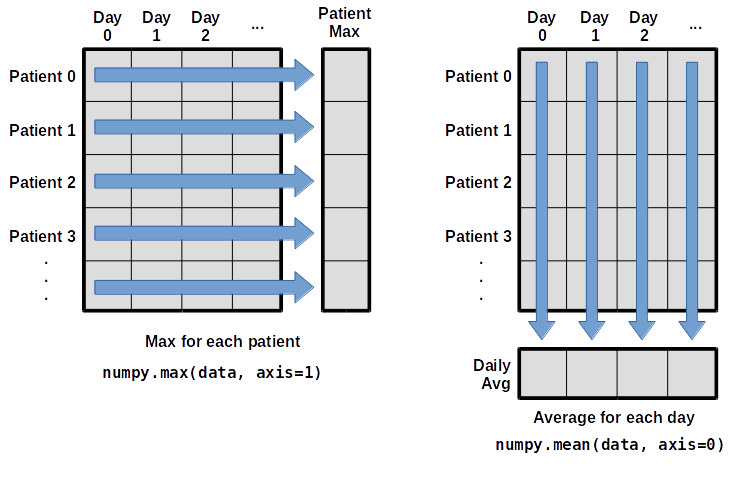
To support this functionality, most array functions allow us to specify the axis we want to work on. If we ask for the average across axis 0 (rows in our 2D example), we get:
OUTPUT
[  0.           0.45         1.11666667   1.75         2.43333333   3.15
   3.8          3.88333333   5.23333333   5.51666667   5.95         5.9
   8.35         7.73333333   8.36666667   9.5          9.58333333
  10.63333333  11.56666667  12.35        13.25        11.96666667
  11.03333333  10.16666667  10.           8.66666667   9.15         7.25
   7.33333333   6.58333333   6.06666667   5.95         5.11666667   3.6
   3.3          3.56666667   2.48333333   1.5          1.13333333
   0.56666667]
As a quick check, we can ask this array what its shape is:
OUTPUT
(40,)The expression (40,) tells us we have an N×1 vector, so
this is the average inflammation per day for all patients. If we average
across axis 1 (columns in our 2D example), we get:
OUTPUT
[ 5.45   5.425  6.1    5.9    5.55   6.225  5.975  6.65   6.625  6.525
  6.775  5.8    6.225  5.75   5.225  6.3    6.55   5.7    5.85   6.55
  5.775  5.825  6.175  6.1    5.8    6.425  6.05   6.025  6.175  6.55
  6.175  6.35   6.725  6.125  7.075  5.725  5.925  6.15   6.075  5.75
  5.975  5.725  6.3    5.9    6.75   5.925  7.225  6.15   5.95   6.275  5.7
  6.1    6.825  5.975  6.725  5.7    6.25   6.4    7.05   5.9  ]
which is the average inflammation per patient across all days.
Slicing Strings
A section of an array is called a slice. We can take slices of character strings as well:
PYTHON
element = 'oxygen'
print('first three characters:', element[0:3])
print('last three characters:', element[3:6])
OUTPUT
first three characters: oxy
last three characters: gen
What is the value of element[:4]? What about
element[4:]? Or element[:]?
OUTPUT
oxyg
en
oxygenSlicing Strings (continued)
What is element[-1]? What is
element[-2]?
OUTPUT
n
eSlicing Strings (continued)
Given those answers, explain what element[1:-1]
does.
Creates a substring from index 1 up to (not including) the final index, effectively removing the first and last letters from ‘oxygen’
Slicing Strings (continued)
How can we rewrite the slice for getting the last three characters of
element, so that it works even if we assign a different
string to element? Test your solution with the following
strings: carpentry, clone,
hi.
PYTHON
element = 'oxygen'
print('last three characters:', element[-3:])
element = 'carpentry'
print('last three characters:', element[-3:])
element = 'clone'
print('last three characters:', element[-3:])
element = 'hi'
print('last three characters:', element[-3:])
OUTPUT
last three characters: gen
last three characters: try
last three characters: one
last three characters: hiThin Slices
The expression element[3:3] produces an empty string, i.e., a string that
contains no characters. If data holds our array of patient
data, what does data[3:3, 4:4] produce? What about
data[3:3, :]?
OUTPUT
array([], shape=(0, 0), dtype=float64)
array([], shape=(0, 40), dtype=float64)Stacking Arrays
Arrays can be concatenated and stacked on top of one another, using
NumPy’s vstack and hstack functions for
vertical and horizontal stacking, respectively.
PYTHON
import numpy

A = numpy.array([[1, 2, 3], [4, 5, 6], [7, 8, 9]])
print('A = ')
print(A)

B = numpy.hstack([A, A])
print('B = ')
print(B)

C = numpy.vstack([A, A])
print('C = ')
print(C)
OUTPUT
A =
[[1 2 3]
 [4 5 6]
 [7 8 9]]
B =
[[1 2 3 1 2 3]
 [4 5 6 4 5 6]
 [7 8 9 7 8 9]]
C =
[[1 2 3]
 [4 5 6]
 [7 8 9]
 [1 2 3]
 [4 5 6]
 [7 8 9]]
Write some additional code that slices the first and last columns of
A, and stacks them into a 3x2 array. Make sure to
print the results to verify your solution.
A ‘gotcha’ with array indexing is that singleton dimensions are
dropped by default. That means A[:, 0] is a one dimensional
array, which won’t stack as desired. To preserve singleton dimensions,
the index itself can be a slice or array. For example,
A[:, :1] returns a two dimensional array with one singleton
dimension (i.e. a column vector).
OUTPUT
D =
[[1 3]
 [4 6]
[7 9]]Change In Inflammation
The patient data is longitudinal in the sense that each row represents a series of observations relating to one individual. This means that the change in inflammation over time is a meaningful concept. Let’s find out how to calculate changes in the data contained in an array with NumPy.
The numpy.diff() function takes an array and returns the
differences between two successive values. Let’s use it to examine the
changes each day across the first week of patient 3 from our
inflammation dataset.
OUTPUT
[0. 0. 2. 0. 4. 2. 2.]Calling numpy.diff(patient3_week1) would do the
following calculations
and return the 6 difference values in a new array.
OUTPUT
array([ 0., 2., -2., 4., -2., 0.])Note that the array of differences is shorter by one element (length 6).
When calling numpy.diff with a multi-dimensional array,
an axis argument may be passed to the function to specify
which axis to process. When applying numpy.diff to our 2D
inflammation array data, which axis would we specify?
Change In Inflammation (continued)
If the shape of an individual data file is (60, 40) (60
rows and 40 columns), what would the shape of the array be after you run
the diff() function and why?
The shape will be (60, 39) because there is one fewer
difference between columns than there are columns in the data.
Change In Inflammation (continued)
How would you find the largest change in inflammation for each patient? Does it matter if the change in inflammation is an increase or a decrease?
By using the numpy.amax() function after you apply the
numpy.diff() function, you will get the largest difference
between days.
PYTHON
array([  7.,  12.,  11.,  10.,  11.,  13.,  10.,   8.,  10.,  10.,   7.,
         7.,  13.,   7.,  10.,  10.,   8.,  10.,   9.,  10.,  13.,   7.,
        12.,   9.,  12.,  11.,  10.,  10.,   7.,  10.,  11.,  10.,   8.,
        11.,  12.,  10.,   9.,  10.,  13.,  10.,   7.,   7.,  10.,  13.,
        12.,   8.,   8.,  10.,  10.,   9.,   8.,  13.,  10.,   7.,  10.,
         8.,  12.,  10.,   7.,  12.])
If inflammation values decrease along an axis, then the
difference from one element to the next will be negative. If you are
interested in the magnitude of the change and not the
direction, the numpy.absolute() function will provide
that.
Notice the difference if you get the largest absolute difference between readings.
PYTHON
array([ 12.,  14.,  11.,  13.,  11.,  13.,  10.,  12.,  10.,  10.,  10.,
        12.,  13.,  10.,  11.,  10.,  12.,  13.,   9.,  10.,  13.,   9.,
        12.,   9.,  12.,  11.,  10.,  13.,   9.,  13.,  11.,  11.,   8.,
        11.,  12.,  13.,   9.,  10.,  13.,  11.,  11.,  13.,  11.,  13.,
        13.,  10.,   9.,  10.,  10.,   9.,   9.,  13.,  10.,   9.,  10.,
11., 13., 10., 10., 12.])- Import a library into a program using
import libraryname. - Use the
numpylibrary to work with arrays in Python. - The expression
array.shapegives the shape of an array. - Use
array[x, y]to select a single element from a 2D array. - Array indices start at 0, not 1.
- Use
low:highto specify aslicethat includes the indices fromlowtohigh-1. - Use
# some kind of explanationto add comments to programs. - Use
numpy.mean(array),numpy.amax(array), andnumpy.amin(array)to calculate simple statistics. - Use
numpy.mean(array, axis=0)ornumpy.mean(array, axis=1)to calculate statistics across the specified axis.